Answers to Exercises
4 R Syntax
# 3.  Calculate the sum of 2 and 3.


2 + 3


# 4.  Evaluate if 0.5 is equal to 1 divided by 2.

0.5 == 1 / 2

# 5.  Define a variable that is is 98.6 degrees in Fahrenheit.

fahrenheit_temp <- 101


# 6.  Construct an if-else statement to determine if the temperature indicates a fever (temperature greater than or equal to 100). If it does print "The temperature indicates a fever." If the temperature is less than 100, print "The temperature does not indicate a fever." (hint: to print "ok", the function is print("ok"))

if (fahrenheit_temp >= 100){
  print("The temperature indicates a fever.")
}else{
  print("The temperature does not indicate a fever.")
}


# 8.  Create a function to test if a temperature is a fever called `fever_checker` the prints above, but can be reused


fever_checker <- function(fahrenheit_temp) {
  if (fahrenheit_temp >= 100){
    print("The temperature indicates a fever.")
  }else{
    print("The temperature does not indicate a fever.")
  }
}


# 9.  Use similar logic to print if a temperature is the homeostatic range for human beings (97.7–99.5).


homeostatic_range_check <- function(fahrenheit_temp){
  if (fahrenheit_temp >= 97.7 && fahrenheit_temp <= 99.5){
    print("In homeostatic range!")
  } else{
    print("Outside homeostatic range!")
  }
}


# 10. Advanced exercise... add TRUE / FALSE returns (i.e. return TRUE, return FALSE) to the functions and create a function that combines both called `temperature_check`. That gives us info on the what our temperature means (i.e., is it homeostatic, is it a fever, are we possibly dead (temperature way too low??)
# ...
5 R Objects
# John Doe
# 2023-06-02
# Institution Inc.
#
# Data Object Exercises

# 1.  Construct the following vector and store as a variable.

str_gbu <- c('red', 'green', 'blue')


# 2.  Extract the 2nd element in the variable.

str_gbu[2]

# 3.  Construct a numerical vector of length 5, containing the AREA of circles
#     with integer RADIUS 1 to 5. Remember PEMDAS.

area <- (1:5) ^ 2 * pi


# 4.  Extract all AREA greater than 50.

area[which(area > 50)]


# 5. Create a data.frame consisting of circles with integer RADIUS 1 to 5, and their AREA.

radius <- 1:5

df <- data.frame(
  radius = radius,
  area = (radius) ^ 2 * pi
)

df


# 6.  Extract all AREA greater than 50 from the data.frame.

w <- which(df$area > 50)
df[w,]
5 R Objects MORE
# John Doe
# 2023-06-02
# Institution Inc.
#
# More Data Object Exercises

# Exercise #1 -- Working with Variables You are running an LC-MS experiment
#     using a 60 min LC gradient

# 1.1 Create a variable called gradient_min to hold the length of the gradient
#     in minutes.

gradient_min <- 60


# 1.2 Using the gradient length variable you just created, convert it to seconds
#     and assign it to a new variable with a meaningful name.

gradient_sec <- gradient_min * 60


# Exercise #2 -- Working with Vectors

# Continuing from Exercise #1...

# 2.1 Imagine you conducted additional experiments, one with a 15 minute gradient
#     and one with a 30 min gradient. Create a vector to hold all three gradient
#     times in minutes, and assign it to a new variable.

gradients_min <- c(15, 30, 60)


# 2.2 Convert the vector of gradient times to seconds. How does this conversion
#     compare to how you did the conversion in Exercise 1?

gradients_sec <- gradients_min * 60


# Exercise #3 -- More Practice with Vectors

# 3.1 The following vector represents precursor m/z values for detected features
#     from your experiment:

prec_mz <- c(968.4759, 812.1599, 887.9829, 338.5294, 510.2720,
             775.3455, 409.2369, 944.0385, 584.7687, 1041.9523)


# -   How many values are there?

length(prec_mz)


# -   What is the minimum value? The maximum?

min(prec_mz)
max(prec_mz)


# Exercise #4 -- Vectors and Conditional Expressions

# 4.1 Using the above vector of precursor values, write a conditional expression
#     to find the values with m/z \< 600. What is returned by this expression? A
#     single value or multiple values? A number or something else?

prec_mz < 600


# 4.2 Use this conditional expression to get the precursor values with m/z \< 600

prec_mz[prec_mz < 600]


# 4.3 Consider a new vector of data that contains the charge states of the same
#     detected features from above:

prec_z <- c(2, 4, 2, 3, 2, 2, 2, 2, 2, 2)


# -   Write a conditional expression to find which detected features that have
#     a charge state of 2.

prec_z == 2


# 4.4 Write an expression to get the precursor m/z values for features having
#     charge states of 2?

prec_mz[prec_z == 2]
6 Tidyverse
- Read in the
bacterial-metabolites_dose-simicillin_tidy.csvdata set.
url <- "https://raw.githubusercontent.com/jeffsocal/ASMS_R_Basics/main/data/bacterial-metabolites_dose-simicillin_tidy.csv"
download.file(url, destfile = "./data/bacterial-metabolites_dose-simicillin_tidy.csv")## Rows: 180 Columns: 5
## ── Column specification ──────────────────────────────────────────────────────
## Delimiter: ","
## chr (2): Organism, Metabolite
## dbl (3): Dose_mg, Time_min, Abundance
##
## ℹ Use `spec()` to retrieve the full column specification for this data.
## ℹ Specify the column types or set `show_col_types = FALSE` to quiet this message.- How many organisms, metabolites, dose levels, and time points are in the data? How many rows are in the data table? What is the overall study design?
orgs <- unique(dat$Organism)
n_orgs <- length(unique(orgs))

metabs <- unique(dat$Metabolite)
n_metabs <- length(unique(metabs))

doses <- unique(dat$Dose_mg)
n_doses <- length(unique(doses))

time_pts <- unique(dat$Time_min)
n_time_pts <- length(unique(time_pts))

nrow(dat)
## [1] 180## [1] TRUE- Which metabolite has the highest overall mean abundance?
dat %>%
  group_by(Metabolite) %>%
  summarize(mean_abundance = mean(Abundance)) %>%
  arrange(desc(mean_abundance))
## # A tibble: 4 × 2
## Metabolite mean_abundance
## <chr> <dbl>
## 1 phosphatidylcholine 50221415.
## 2 succinic acid 1855206.
## 3 glutamate 1817320.
## 4 lysine 1349963.- Does this metabolite have the highest mean abundance for each organism, or is there differences between organisms?
dat %>%
  group_by(Organism, Metabolite) %>%
  summarize(mean_abundance = mean(Abundance)) %>%
  arrange(Organism, desc(mean_abundance))
## `summarise()` has grouped output by 'Organism'. You can override using the
## `.groups` argument.## # A tibble: 12 × 3
## # Groups: Organism [3]
## Organism Metabolite mean_abundance
## <chr> <chr> <dbl>
## 1 e coli phosphatidylcholine 67749754.
## 2 e coli glutamate 2323045.
## 3 e coli succinic acid 1906850.
## 4 e coli lysine 1519827.
## 5 p aeruginosa phosphatidylcholine 77078132.
## 6 p aeruginosa succinic acid 3525432.
## 7 p aeruginosa glutamate 2902178
## 8 p aeruginosa lysine 2336119.
## 9 staph aureus phosphatidylcholine 5836359.
## 10 staph aureus glutamate 226736.
## 11 staph aureus lysine 193944.
## 12 staph aureus succinic acid 133337.- Is there an overall trend of mean abundance values vs. time point? What about abundance vs. dose?
## # A tibble: 5 × 2
##   Time_min mean_abundance
##      <dbl>          <dbl>
## 1        0      26639946.
## 2       10      11726915.
## 3       20      11929517.
## 4       50       9389061.
## 5 120 9369441.## # A tibble: 3 × 2
## Dose_mg mean_abundance
## <dbl> <dbl>
## 1 0 24454975.
## 2 10 9900030.
## 3 20 7077924.- Using the example code at the beginning of this Chapter (using the Dever climate data), compute a linear fit of log10 abundance vs. time point for each metabolite and plot the results.
dat <- dat %>%
  mutate(log10_abundance = log10(Abundance))

lm_func <- function(data) {
  lm(log10_abundance ~ Time_min, data = data)
}


dat_lm <- dat %>%
  # dplyr
  group_by(Metabolite) %>%
  # tidyr
  nest() %>%
  # dplyr, purrr: apply the function to each nested data frame
  mutate(model = map(data, lm_func)) %>%
  # dplyr, broom, purrr: extract the coefficients from each model
  mutate(tidy = map(model, broom::tidy)) %>%
  # tidyr
  unnest(tidy) %>%
  ungroup() %>%
  # dplyr, stringr: clean-up the terms
  mutate(term = term %>% str_replace_all("\\(|\\)", "")) %>%
  # dplyr: retain only specific columns
  select(Metabolite, term, estimate) %>%
  # tidyr: convert from a long table to a wide table
  pivot_wider(names_from = 'term', values_from = 'estimate') %>%
  # dplyr: create a new column with the model slope (better name), just copy Time_min
  mutate(model_slope = Time_min)


#ggplot2
ggplot(dat, aes(Time_min, log10_abundance)) +
  # represent the data as points
  geom_point() +
  # use the linear model data to plot regression lines
  geom_abline(data = dat_lm,
              aes(slope = model_slope, intercept = Intercept)) +
  # plot each year separately
  facet_wrap(~Metabolite)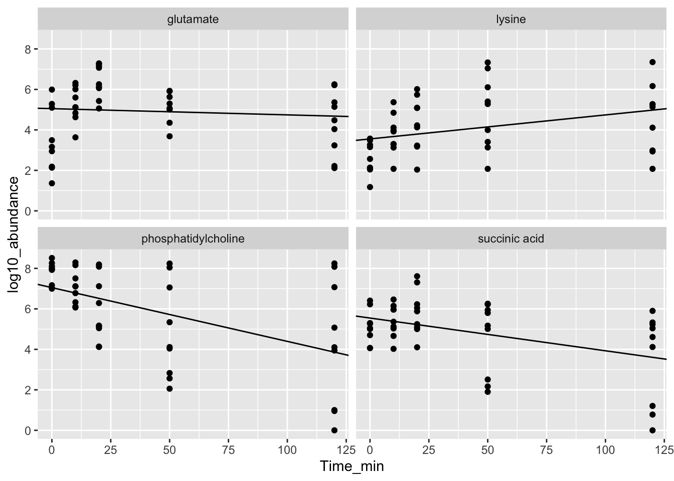
7 Data Wrangling
# John Doe
# 2023-06-02
# Institution Inc.
#
# Data Wrangling Exercises

# 1. Download the data.

url <- "https://raw.githubusercontent.com/jeffsocal/ASMS_R_Basics/main/data/bacterial-Metabolites_dose-simicillin_messy.xlsx"
download.file(url, destfile = "./data/bacterial-Metabolites_dose-simicillin_messy.xlsx")


# 2. Read in the messy bacteria data and store it as a variable.

library(tidyverse)
library(readxl)

tbl_bac <- "data/bacterial-Metabolites_dose-simicillin_messy.xlsx" %>% read_excel(col_names = TRUE)


# *In all proceeding exercises, pipe results from previous exercise into current
#    exercise creating a single lone pipe for data processing*

# 3. Separate `Culture` column containing culture and dose into `culture` and
#    `dose_mg_ml` columns.

tbl_bac %>%
  separate(Culture, c("culture", "dose_mg_ml"), sep = " dose--")


# 4. Make `dose_mg_ml` column numeric by removing the text and change the column
#    data type from character to numeric.

tbl_bac %>%
  separate(Culture, c("culture", "dose_mg_ml"), sep = " dose--") %>%
  mutate(dose_mg_ml = gsub("-mg/ml","", dose_mg_ml)) %>%
  mutate(dose_mg_ml = as.numeric(dose_mg_ml))


# 5. Pivot the table from wide to long creating `metabolite`, `time_hr` & `abundance` columns.

tbl_bac %>%
  separate(Culture, c("culture", "dose_mg_ml"), sep = " dose--") %>%
  mutate(dose_mg_ml = gsub("-mg/ml","", dose_mg_ml)) %>%
  mutate(dose_mg_ml = as.numeric(dose_mg_ml)) %>%
  pivot_longer(cols = 4:13, names_to = "metabolite_time", values_to = "abundance") %>%
  separate(metabolite_time, c("metabolite","time_hr"), sep="_runtime_")


# 6. Make sure `time_hr` contains just hours and not a mixture of days and hours.

tbl_bac %>%
  separate(Culture, c("culture", "dose_mg_ml"), sep = " dose--") %>%
  mutate(dose_mg_ml = gsub("-mg/ml","", dose_mg_ml)) %>%
  mutate(dose_mg_ml = as.numeric(dose_mg_ml)) %>%
  pivot_longer(cols = 4:13, names_to = "metabolite_time", values_to = "abundance") %>%
  separate(metabolite_time, c("metabolite","time_hr"), sep="_runtime_") %>%
    mutate(
    time_hr = case_when(
      grepl("hr", time_hr, ignore.case = TRUE) ~ as.numeric(gsub("hr", "", time_hr)),
      grepl("day", time_hr, ignore.case = TRUE) ~ as.numeric(gsub("day", "", time_hr)) * 24
    )
  )


# 7. Remove the `User` column. See the cheat-sheet here:
#    https://www.rstudio.com/wp-content/uploads/2015/02/data-wrangling-cheatsheet.pdf

tbl_bac %>%
  separate(Culture, c("culture", "dose_mg_ml"), sep = " dose--") %>%
  mutate(dose_mg_ml = gsub("-mg/ml","", dose_mg_ml)) %>%
  mutate(dose_mg_ml = as.numeric(dose_mg_ml)) %>%
  pivot_longer(cols = 4:13, names_to = "metabolite_time", values_to = "abundance") %>%
  separate(metabolite_time, c("metabolite","time_hr"), sep="_runtime_") %>%
    mutate(
    time_hr = case_when(
      grepl("hr", time_hr, ignore.case = TRUE) ~ as.numeric(gsub("hr", "", time_hr)),
      grepl("day", time_hr, ignore.case = TRUE) ~ as.numeric(gsub("day", "", time_hr)) * 24
    )
  ) %>%
  select(-User)
8 Data Visualization
# John Doe
# 2023-06-02
# Institution Inc.
#
# Data Visualization Exercises

# 1. If not already done, download *Bacterial Metabolite Data (tidy)* to use as
#    an example data file.

url <- "https://raw.githubusercontent.com/jeffsocal/ASMS_R_Basics/main/data/bacterial-Metabolites_dose-simicillin_tidy.csv"
download.file(url, destfile = "./data/bacterial-Metabolites_dose-simicillin_tidy.csv")


# 2. Read in the dataset .csv using the `tidyverse` set of packages.

library(tidyverse)

tbl_bac <- "./data/bacterial-Metabolites_dose-simicillin_tidy.csv" %>% read_csv()


# 3. Create a Metabolite `Abundance` by `Time_min` ...

tbl_bac %>%
  ggplot(aes(Time_min, Abundance)) +
  geom_point()


# 4. ... facet by `Organism` and `Metabolite`...

tbl_bac %>%
  ggplot(aes(Time_min, Abundance)) +
  geom_point() +
  facet_grid(Metabolite ~ Organism)


# 4. ... adjust the y-axis to log10, color by `Dose_mg`, and add a 50% transparent line ...

tbl_bac %>%
  mutate(Dose_mg = Dose_mg %>% as.factor()) %>%
  ggplot(aes(Time_min, Abundance)) +
  geom_point(aes(color = Dose_mg)) +
  geom_line(aes(color = Dose_mg), alpha = .5) +
  facet_grid(Metabolite ~ Organism) +
  scale_y_log10()


# 5. ... change the theme to something publishable, add a title, modify the x-
#    and y-axis label, modify the legend title, adjust the y-axis ticks to show
#    the actually measured time values, and pick a color scheme that highlights
#    the dose value...

tbl_bac %>%
  mutate(Dose_mg = Dose_mg %>% as.factor()) %>%
  ggplot(aes(Time_min, Abundance)) +
  geom_point(aes(color = Dose_mg)) +
  geom_line(aes(color = Dose_mg), alpha = .5) +
  facet_grid(Metabolite ~ Organism) +
  scale_color_manual(values = c("grey", "orange", "red")) +
  scale_y_log10() +
  scale_x_continuous(breaks = unique(tbl_bac$Time_min)) +
  labs(title = 'Bacterial Metabolite monitoring by LCMS in response to antibiotic',
       subtitle = 'Conditions: metered dose of similicillin',
       x = "Time (min)", y = "LCMS Abundance",
       color = "Dose (mg)") +
  theme_classic()