Chapter 5 R Objects

The R programming environment includes four basic types of data structures that increase in complexity: variable, vector, matrix, and list. Additionally there is the data.frame while and independent data structure, it is essentially derived from the matrix.

At the end of this chapter you should be able to

Understand the 5 most common data structures.
Understand the data structure lineage.
Access given subsets of a multi-variable data object.

This book introduced variables briefly in 8.2.1. Here, we will expand on that introduction. At its simplest, a variable can be thought of as a container that holds only a single thing, like a single stick of gum. A vector is an ordered, finite collection of variables, like a pack of gum. A matrix consists of columns of equally-sized vectors, similar to a vending machine for several flavors of gum packs. Mentally, you can think of them as a point, a line, and a square, respectively.

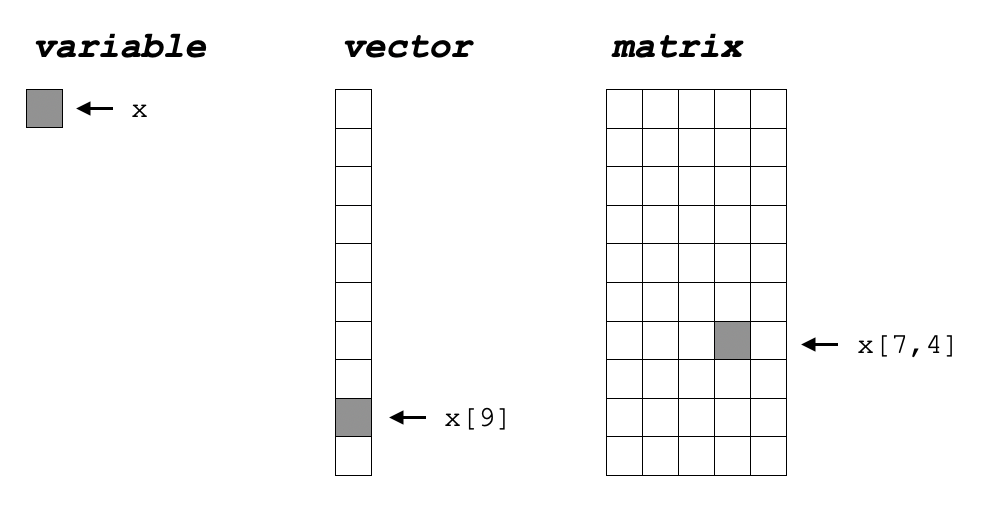
$\label{fig:5001}R main data structures$

Figure 5.1: R main data structures

5.1 Variable

Again, a variable is the most basic information container, capable of holding only a single numeric or string value.

a <- 1

5.2 Vector

A vector is simply a collection of variables of all the same type. In other programming languages these are called arrays, and can be more permissive allowing for different types of values to be stored together. In R this is not permitted, as vectors can only contain either numbers or strings. If a vector contains a single string value, this “spoils” the numbers in the vector, thus making them all strings.

# permitted
a <- c(1, 2, 3)
a

## [1] 1 2 3

# the numerical values of 1 and 3 are lost, and now only represented as strings
b <- c(1, 'two', 3)
b

## [1] "1"   "two" "3"

Vectors can be composed through various methods, either by concatenation with the c() function, as seen above, or using the range operator :. Note that the concatenation method allows for the non-sequential construction of variables, while the range operator constructs a vector of all sequential integers between the two values.

1:3

## [1] 1 2 3

There are also a handful of pre-populated vectors and functions for constructing patters.

# all upper case letters
LETTERS

##  [1] "A" "B" "C" "D" "E" "F" "G" "H" "I" "J" "K" "L" "M" "N" "O" "P" "Q" "R" "S" "T" "U" "V" "W" "X" "Y" "Z"

# all lower case letters
letters

##  [1] "a" "b" "c" "d" "e" "f" "g" "h" "i" "j" "k" "l" "m" "n" "o" "p" "q" "r" "s" "t" "u" "v" "w" "x" "y" "z"

# a repetitive vector of the letter "a"
rep('a', 5)

## [1] "a" "a" "a" "a" "a"

# a repetitive vector of a previous vector
rep(b, 2)

## [1] "1"   "two" "3"   "1"   "two" "3"

# a sequence of integers between two values, in this case reverse order
seq(10, 5)

## [1] 10  9  8  7  6  5

# same as above
10:5

## [1] 10  9  8  7  6  5

While variables don’t require a referencing scheme, because they only contain a single value, vectors need to have some kind of referencing scheme, shown in 5.1 as x[9] and illustrated in the following example.

The use of an integer vector to sub-select another vector based on position. R abides by the 1:N positional referencing, where as other programming languages refer to the first vector or array position as 0. A good topic for a lively discussion with a computer scientist.

x <- LETTERS
# 3rd letter in the alphabet
x[3]

## [1] "C"

# the 9th, 10th, 11th and 12th letters in the alphabet
x[9:12]

## [1] "I" "J" "K" "L"

# the 1st, 5th, 10th letters in the alphabet
x[c(1,5,10)]

## [1] "A" "E" "J"

Numerical vectors can be operated on simultaneously, using the same conventions as variables, imparting convenient utlity to calculating on collections of values.

x <- 1:10
x / 10

##  [1] 0.1 0.2 0.3 0.4 0.5 0.6 0.7 0.8 0.9 1.0

In addition, there are facile ways to extract information using a coonditional statement …

x <- 1:10 / 10
x < .5

##  [1]  TRUE  TRUE  TRUE  TRUE FALSE FALSE FALSE FALSE FALSE FALSE

… the which() function returns the integer reference positions for the condition x < 0.5 …

which(x < .5)

## [1] 1 2 3 4

… and since the output of that function is a vector, we can use it to reference the original vector to extract the elements in the vector that satisfy our condition x < 0.5.

x[which(x < .5)]

## [1] 0.1 0.2 0.3 0.4

5.3 List

In R programming, a ‘list’ is a powerful and flexible collection of objects of different types. It can contain vectors, matrices, data frames, and even other lists, making it an extremely versatile tool in data analysis, modeling, and visualization.

With its ability to store multiple data types, a list can be used to represent complex structures such as a database table, where each column can be a vector or a matrix. Furthermore, a list can be used to store multiple models for model comparison, or to store a set of parameters for a simulation study.

In addition to its flexibility, a list is also efficient, as it allows for fast and easy data retrieval. It can be used to store large datasets, and its hierarchical structure makes it easy to navigate and manipulate.

Here’s an example of how to create a list in R:

# create a list
my_list <- list(name = "Janie R Programmer",
                age = 32,
                salary = 100000,
                interests = c("coding", "reading", "traveling"))

print(my_list)

## $name
## [1] "Janie R Programmer"
## 
## $age
## [1] 32
## 
## $salary
## [1] 1e+05
## 
## $interests
## [1] "coding"    "reading"   "traveling"

In the above code, we have created a list ‘my_list’ with four elements, each having a different data type. The first element ‘name’ is a character vector, the second element ‘age’ is a numeric value, the third element ‘salary’ is also a numeric value, and the fourth element ‘interests’ is a character vector.

We can access the elements of a list using the dollar sign ‘$’ or double brackets ‘[[]]’. For example:

# accessing elements of a list
print(my_list$name)

## [1] "Janie R Programmer"

print(my_list[["salary"]])

## [1] 1e+05

Lists are also useful for storing and manipulating complex data structures such as data frames and tibbles.

5.4 Matrix

Building upon the vector, a matrix is simply composed of columns of either all numeric or string vectors. That statement is not completely accurate as matrices can be row based, however, if we mentally orient ourselves to column based organizations, then the following data.frame will make sense. Matrices are constructed using a function as shown in the following example.

# taking the vector 1:4 and distributing it by 2 rows and 2 columns
m <- matrix(1:4,2,2)

Elements within the matrix have a reference schema similar to vectors, with the first integer in the square brackets is the row and the second the column [row,col].

##      [,1] [,2]
## [1,]    1    3
## [2,]    2    4

Just like a vector, a matrix can be used to compute operations on all elements simultaneously, apply a comparison and extract the variable(s) matching the condition …

m_half <- m / 2
w_point5 <- which(m_half > 1)
m[w_point5]

## [1] 3 4

… or more sincintly.

m[which(m/2 > 1)]

## [1] 3 4

5.5 Data Frame

Tables are one of the fundamental data structures encountered in data analysis, and what separates them from matrices is the mixed use of numerics and strings, and the orientation that data.frames are columns of vectors, with a row association. A table can be cinstructed with the data.frame() function as shown in the example.

df <- data.frame(
  let = LETTERS,
  pos = 1:length(LETTERS)
)

##    let pos
## 1    A   1
## 2    B   2
## 3    C   3
## 4    D   4
## 5    E   5
## ...

Lets talk about the structure of what just happened in constructing the data.frame table. Note that we defined the column with let and pos referring to letter and position, respectively. Second, note the use of the single = to assign a vector to that column rather than the “out-of-function” assignment operator <- – meaning that functions use the = assignment operator, while data structures use the <- assignment operator.

The printed output of the data.frame shows the two column headers and also prints out the row names, in this case the integer value. Now, that this table is organized by column with row assiciations, we can perform an evalutaion on one column and reterive the value(s) in the other.

5.6 Data Table

A data.table is a package in R that provides an extension of data.frame. It is an optimized and efficient way of handling large datasets in R language. Data.table is widely used in data science as it provides fast and easy ways to analyze large datasets. It is built to handle large datasets with ease while still providing a simple and intuitive syntax. Some R packages build specifically for mass spectrometry utilize data.tables, however, its is easy to transform between object types and use the methods you are most comfortable with.

The data.table object provides many advantages over the traditional data.frame. Some of the key advantages are as follows:

Faster performance as compared to data.frame.
Efficient memory usage.
Provides an easy way to handle and manipulate large datasets.
Provides a syntax similar to SQL for easy querying of data.

library(data.table)

tbl_let <- data.table(
  let = LETTERS,
  pos = 1:length(LETTERS)
)

##     let pos
##  1:  A   1
##  2:  B   2
##  3:  C   3
##  4:  D   4
##  5:  E   5
## ...
## 26:   Z  26
##     let pos

In addition, data.table also provides many functions for data manipulation and aggregation. Some of the commonly used functions are:

.SD: Subset of Data.table. It is used to access the subset of data.table.
.N: It is used to get the number of rows in a group.
.SDcols: It is used to select columns to subset .SD.
.GRP: It is used to get the group number of each row.

5.7 Tibbles

A tibble is a modern data frame in R programming language. Tibble is a part of tidyverse package that provides an efficient and user-friendly way to work with data frames. Tibbles are similar to data frames, but they have better printing capabilities, and they are designed to never alter your data.

Tibbles are created using the tibble() function. You can create a tibble by passing vectors, lists, or data frames to the tibble() function. Once created, you can manipulate the tibble using the dplyr package.

library(tidyverse)

tbl_let <- tibble(
  let = LETTERS,
  pos = 1:length(LETTERS)
)

## # A tibble: 26 × 2
##    let     pos
##    <chr> <int>
##  1 A         1
##  2 B         2
##  3 C         3
##  4 D         4
##  5 E         5
##  6 F         6
##  7 G         7
##  8 H         8
##  9 I         9
## 10 J        10
## # … with 16 more rows
## # ℹ Use `print(n = ...)` to see more rows

Tibbles have several advantages over data frames. They print only the first 10 rows and all the columns that fit on the screen. This makes it easier to view and work with large datasets. Tibbles also have better error messages, which makes debugging easier. Additionally, tibbles are more consistent in handling columns with different types of data.

Examine the Contents

You can use the str() function to peak inside any data object to see how it is structured.

The contents of a data.frame:

plant_data <- data.frame(
  age_days = c(10, 20, 30, 40, 50, 60),
  height_inch = c(1.02, 1.10, 5.10, 6.00, 6.50, 6.90)
)

str(plant_data)

## 'data.frame':    6 obs. of  2 variables:
##  $ age_days   : num  10 20 30 40 50 60
##  $ height_inch: num  1.02 1.1 5.1 6 6.5 6.9

The contents of a tibble is very similar:

plant_data <- data.table(
  age_days = c(10, 20, 30, 40, 50, 60),
  height_inch = c(1.02, 1.10, 5.10, 6.00, 6.50, 6.90)
)

str(plant_data)

## Classes 'data.table' and 'data.frame':   6 obs. of  2 variables:
##  $ age_days   : num  10 20 30 40 50 60
##  $ height_inch: num  1.02 1.1 5.1 6 6.5 6.9
##  - attr(*, ".internal.selfref")=<externalptr>

The contents of a tibble is very similar:

plant_data <- tibble(
  age_days = c(10, 20, 30, 40, 50, 60),
  height_inch = c(1.02, 1.10, 5.10, 6.00, 6.50, 6.90)
)

str(plant_data)

## tibble [6 × 2] (S3: tbl_df/tbl/data.frame)
##  $ age_days   : num [1:6] 10 20 30 40 50 60
##  $ height_inch: num [1:6] 1.02 1.1 5.1 6 6.5 6.9

The contents of a linear regression data object are quite different:

# linear prediction of plant growth (eg. height) based on age
linear_model <- lm(data = plant_data, height_inch ~ age_days)

linear_model

## 
## Call:
## lm(formula = height_inch ~ age_days, data = plant_data)
## 
## Coefficients:
## (Intercept)     age_days  
##     -0.2133       0.1329

str(linear_model)

List of 12
 $ coefficients : Named num [1:2] -0.213 0.133
  ..- attr(*, "names")= chr [1:2] "(Intercept)" "age_days"
 $ residuals    : Named num [1:6] -0.0952 -1.3438 1.3276 0.899 0.0705 ...
  ..- attr(*, "names")= chr [1:6] "1" "2" "3" "4" ...
 $ effects      : Named num [1:6] -10.868 5.558 1.296 0.602 -0.492 ...
  ..- attr(*, "names")= chr [1:6] "(Intercept)" "age_days" "" "" ...
 $ rank         : int 2
 $ fitted.values: Named num [1:6] 1.12 2.44 3.77 5.1 6.43 ...
  ..- attr(*, "names")= chr [1:6] "1" "2" "3" "4" ...

Converting Objects

In R, we see that there are several data objects that can be used to store and manipulate data. Some of the commonly used data objects include data.frames, data.tables and tibbles. However, we don’t need to be stuck with any one object and can easily convert between these data objects using the as.data.frame, as.data.table and as_tibble functions.

If we start out with a data.frame as shown above, we can convert that to either a data.table or a tibble very easily.

library(tibble)
library(data.table)

Convert from a data.frame to a data.table:

dt <- as.data.table(df)
str(dt)

## Classes 'data.table' and 'data.frame':   26 obs. of  2 variables:
##  $ let: chr  "A" "B" "C" "D" ...
##  $ pos: int  1 2 3 4 5 6 7 8 9 10 ...
##  - attr(*, ".internal.selfref")=<externalptr>

Convert from a data.frame to a tibble:

tbl <- as_tibble(df)
str(tbl)

## tibble [26 × 2] (S3: tbl_df/tbl/data.frame)
##  $ let: chr [1:26] "A" "B" "C" "D" ...
##  $ pos: int [1:26] 1 2 3 4 5 6 7 8 9 10 ...

Convert from a data.table to a tibble:

tbl <- as_tibble(dt)
str(tbl)

## tibble [26 × 2] (S3: tbl_df/tbl/data.frame)
##  $ let: chr [1:26] "A" "B" "C" "D" ...
##  $ pos: int [1:26] 1 2 3 4 5 6 7 8 9 10 ...
##  - attr(*, ".internal.selfref")=<externalptr>

Exercises

Create a new R Studio Project and name it 003_data_structures.
Create a new R script, add your name and date at the top as comments.

Construct the following vector and store as a variable.

## [1] "red"   "green" "blue"

Extract the 2nd element in the variable.

## [1] "green"

Construct a numerical vector of length 5, containing the AREA of circles with integer RADIUS 1 to 5. Remember PEMDAS.

## [1]  3.141593 12.566372 28.274337 50.265488 78.539825

Extract all AREA greater than 50.

## [1] 50.26549 78.53982

Create a data.frame consisting of circles with integer RADIUS 1 to 5, and their AREA.

##   radius      area
## 1      1  3.141593
## 2      2 12.566372
## 3      3 28.274337
## 4      4 50.265488
## 5      5 78.539825

Extract all AREA greater than 50 from the data.frame.

##   radius     area
## 4      4 50.26549
## 5      5 78.53982

More Exercises

Create a new R Studio Project and name it 103_data_structures.
Create a new R script, add your name and date at the top as comments.

Exercise #1 – Working with Variables You are running an LC-MS experiment using a 60 min LC gradient

1.1 Create a variable called gradient_min to hold the length of the gradient in minutes.

## [1] 60

1.2 Using the gradient length variable you just created, convert it to seconds and assign it to a new variable with a meaningful name.

## [1] 3600

Exercise #2 – Working with Vectors

Continuing from Exercise #1…

2.1 Imagine you conducted additional experiments, one with a 15 minute gradient and one with a 30 min gradient. Create a vector to hold all three gradient times in minutes, and assign it to a new variable.

## [1] 15 30 60

2.2 Convert the vector of gradient times to seconds. How does this conversion compare to how you did the conversion in Exercise 1?

## [1]  900 1800 3600

Exercise #3 – More Practice with Vectors

3.1 The following vector represents precursor m/z values for detected features from your experiment:

prec_mz <- c(968.4759, 812.1599, 887.9829, 338.5294, 510.2720, 
             775.3455, 409.2369, 944.0385, 584.7687, 1041.9523)

How many values are there?

## [1] 10

What is the minimum value? The maximum?

## [1] 338.5294

## [1] 1041.952

Exercise #4 – Vectors and Conditional Expressions

4.1 Using the above vector of precursor values, write a conditional expression to find the values with m/z < 600. What is returned by this expression? A single value or multiple values? A number or something else?

##  [1] FALSE FALSE FALSE  TRUE  TRUE FALSE  TRUE FALSE  TRUE FALSE

4.2 Use this conditional expression to get the precursor values with m/z < 600

## [1] 338.5294 510.2720 409.2369 584.7687

4.3 Consider a new vector of data that contains the charge states of the same detected features from above:

prec_z <- c(2, 4, 2, 3, 2, 2, 2, 2, 2, 2)

Write a conditional expression to find which detected features that have a charge state of 2.

##  [1]  TRUE FALSE  TRUE FALSE  TRUE  TRUE  TRUE  TRUE  TRUE  TRUE

4.4 Write an expression to get the precursor m/z values for features having charge states of 2?

## [1]  968.4759  887.9829  510.2720  775.3455  409.2369  944.0385  584.7687 1041.9523