Imputing

Along with normalization, imputing missing values is another important task in quantitative proteomics that can be challenging to implement given the desired method. Again, tidyproteomics attempts to facilitate this with the impute() function, which currently can support any base level or user defined function along with implementing the R package missForest, widely regarded as one of the best algorithms for missing value imputation. Note that this method is a matrix based sample imputation.

While random forest algorithms have shown superiority in imputation and regression, that does not portend their use in every case. For example, imputing missing values from a knock-out experiment, such as the dataset included in this package, are preferrable to minimum value imputation over the more complex random forest, simply because in this experiment we know how the experiment is affected.

Imputation in tidyproteomics attempts to apply each function universally, meaning the same towards peptide and protein values. To do this each data-object contains a variable called the identifier , this tells the underlying helper functions what values in the quantitative table “identify” the thing being measured.

Proteins have a single identifier …

hela_proteins$identifier
#> [1] "protein"
hela_proteins$quantitative %>% head()
#> # A tibble: 6 × 5
#>   sample_id sample    replicate protein abundance_raw
#>   <chr>     <chr>     <chr>     <chr>           <dbl>
#> 1 9e6ed3ba  control   1         Q15149    1011259992.
#> 2 cc56fc1d  control   2         Q15149    1093277593.
#> 3 6a21f7a9  control   3         Q15149     980809516.
#> 4 966be57f  knockdown 1         Q15149    1410445367.
#> 5 79a98e41  knockdown 2         Q15149    1072305561.
#> 6 9f804505  knockdown 3         Q15149    1486561518.

Peptides have multiple identifiers …

hela_peptides$identifier
#> [1] "protein"       "peptide"       "modifications"
hela_peptides$quantitative %>% head()
#> # A tibble: 6 × 7
#>   sample_id sample  replicate protein peptide        modifications abundance_raw
#>   <chr>     <chr>   <chr>     <chr>   <chr>          <chr>                 <dbl>
#> 1 74a86daf  control 1         P06576  IPSAVGYQPTLAT… NA                43217337 
#> 2 74a86daf  control 1         P06576  IPSAVGYQPTLAT… 1xOxidation …      1465426.
#> 3 74a86daf  control 1         Q9P2E9  LTAEFEEAQTSACR 1xCarbamidom…      5899490.
#> 4 74a86daf  control 1         P11021  ITPSYVAFTPEGER NA                52886668 
#> 5 74a86daf  control 1         P11021  IINEPTAAAIAYG… NA               244628414.
#> 6 74a86daf  control 1         Q9P2E9  LLATEQEDAAVAK  NA                 5831700.

Imputation Functions

Imputation currently supports the following functions:

Function	Method	Description
base::min	row or column	the minimum value in any given set
stats::median	row or column	the minimum value in any given set
user supplied function	any	e.g. function (x, na.rm) { quantile(x, 0.05, na.rm = na.rm)[1] }
impute.knn	matrix only	a non-linear KNN implementation (bioconductor::impute)
impute.randomforest	matrix only	a non-linear random forest implementation of missForest

library("dplyr")
library("ggplot2")
library("tidyproteomics")

# path_to_package_data() loads data specific to this package
# for your project load local data
# example: 
# your_proteins <- "./data/your_exported_results.xlsx" %>%
#   import("ProteomeDiscoverer", "proteins")

rdata <- hela_proteins

As part of this demonstration, signal from P06576 in p07_kd has been artificially removed to simulate a “genetic knockout mutation”.

w <- which(rdata$quantitative$protein == 'P06576' & rdata$quantitative$sample == 'knockdown')
rdata$quantitative <- rdata$quantitative[-w,]

Using column

Note the difference using column ..


rdata %>% 
  impute(.function = base::min, method = 'column') %>%
  subset(protein %like% "P23443|P51812|P06576") %>% 
  extract() %>%
  ggplot(aes(replicate, abundance)) +
  geom_point(aes(color=sample), size=3, alpha=.5) +
  facet_wrap(~identifier) +
  scale_y_log10(limits = c(1e4,1e9)) +
  scale_color_manual(values = c('red','blue'))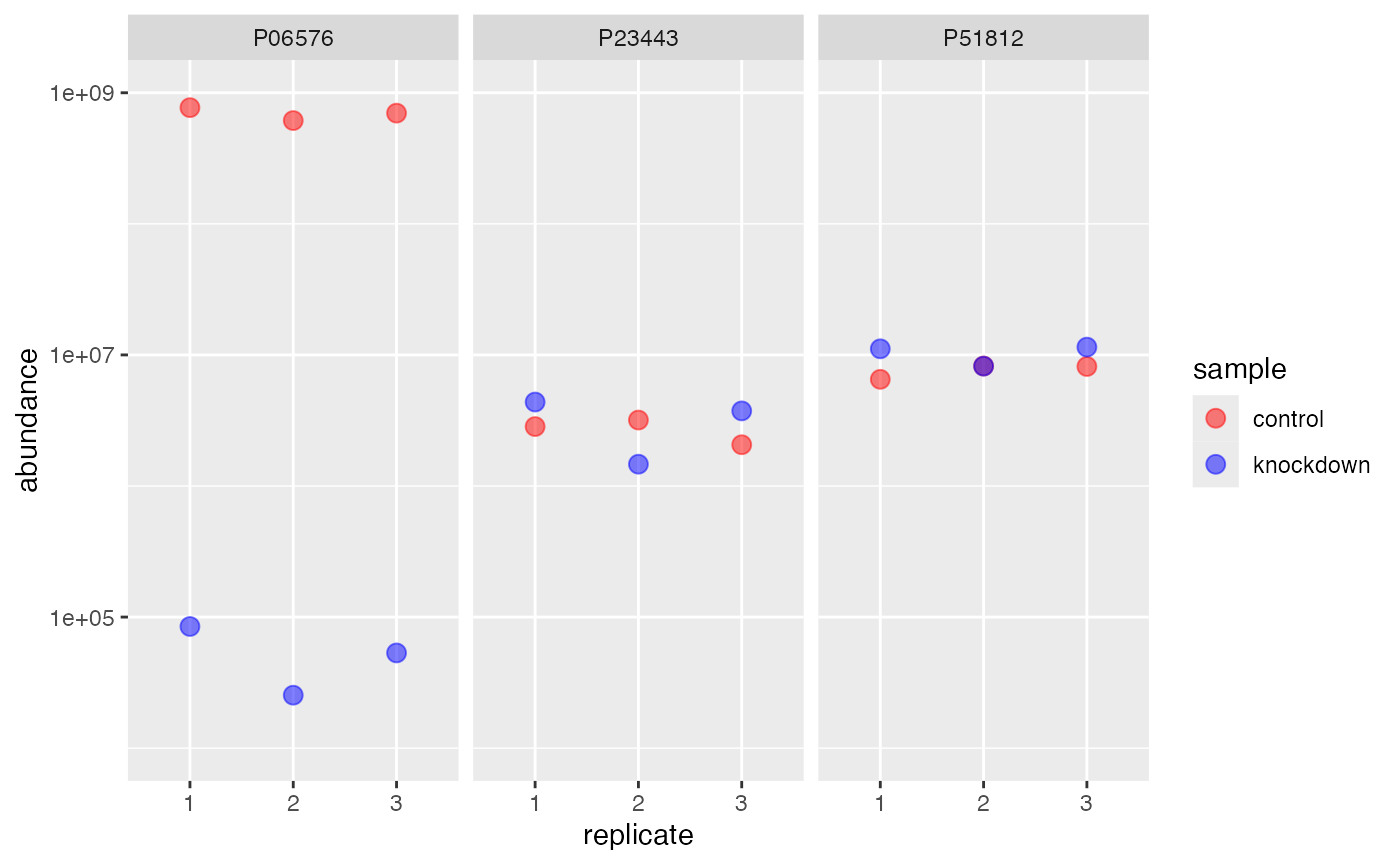

Using row

.. as opposed to row. The row method can be considered to contain the bias of any real offset, note our protein P06576 (i.e our artifical knock-out), shows the expected offset for the column method, and does not for the row method. Consider only using row methods when imputing values you suspect are missing-at-random. In our case P06576 is missing-not-at-random, because we performed a “genetic knockout mutation”.


rdata %>% 
  impute(.function = base::min, method = 'row') %>%
  subset(protein %like% "P23443|P51812|P06576") %>% 
  extract() %>%
  ggplot(aes(replicate, abundance)) +
  geom_point(aes(color=sample), size=3, alpha=.5) +
  facet_wrap(~identifier) +
  scale_y_log10(limits = c(1e4,1e9)) +
  scale_color_manual(values = c('red','blue'))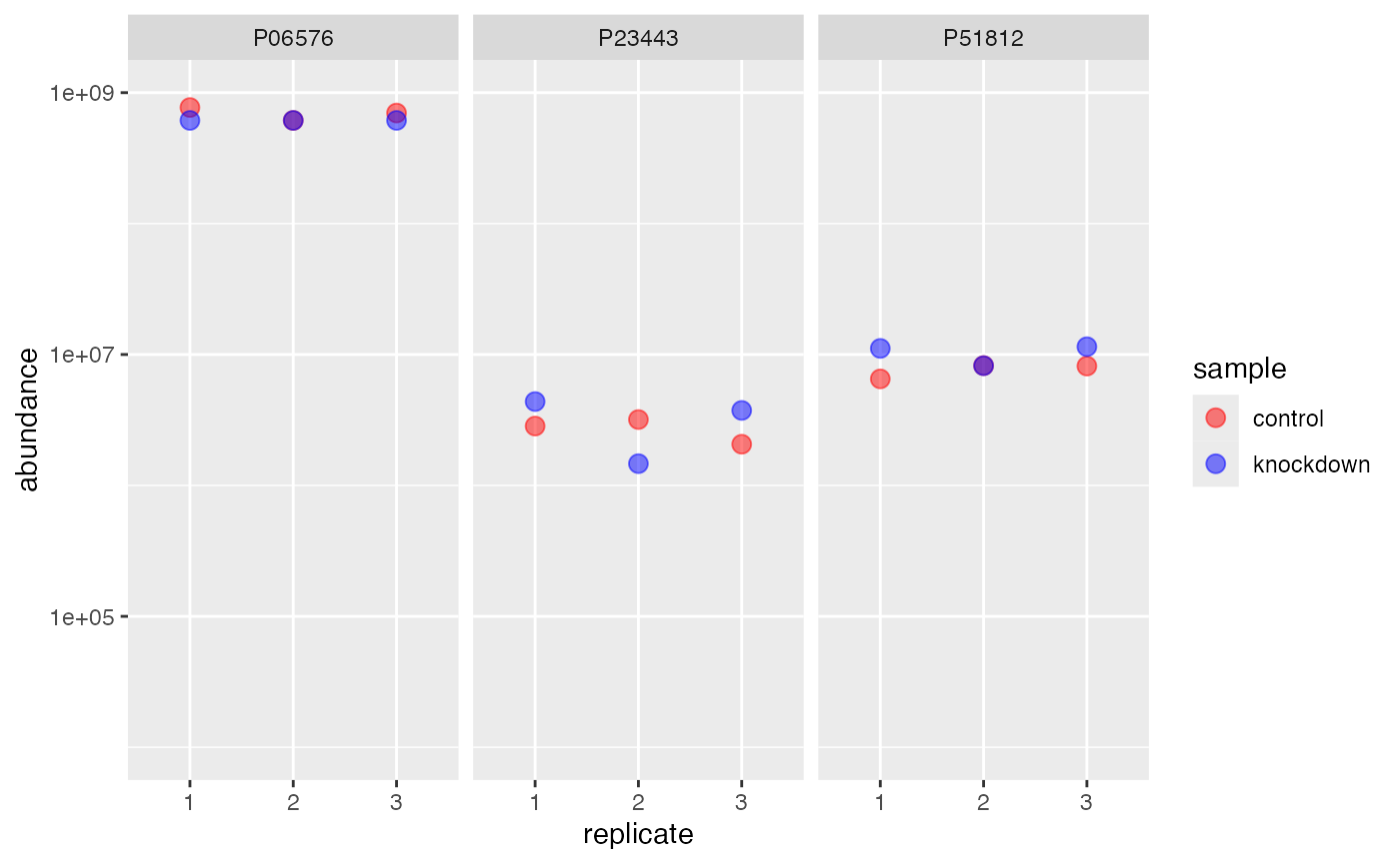

Using matrix

The matrix based operation takes advantage of data present in other samples (eg. “row”) and the information contained in the dynamic range (eg “column”) to better estimate the missing value - usually this is best for missing-at-random.


rdata %>% impute(.function = impute.randomforest, method = 'matrix')

The R package in bioconductor::impute, allows for the popular imputation method KNN. The generalized impute function for the method matrix assumes the underlying function is multithreaded, as is the impute.randomforest method is. Therefore, to make any function operable, you need to make a wrapper function to allow for the cores variable to be accepted. In addition, the impute package returns an incompatible data object, that you must convert to a matrix - fortunately, the impute package’s data object contains the matrix in $data.

library(impute)

my.impute.knn <- function(x, cores = NULL){
  result <- x %>% impute.knn()
  return(result$data)
}

rdata %>% impute(.function = my.impute.knn, method = 'matrix')