Normalizing

Quantitative proteomics relies on accurate normalization, for which several choices are available, yet remain somewhat difficult to accurately implement or require formatting data differently for each. For example, a simple alignment of measured median’s requires only a few lines of code, while implementing normalization from the limma package requires non-intuitive formatting of the data. The normalize() function is designed as a wrapper to handle various methods of normalization all at once, then allowing researchers the ability to examine the result and choose the method best suited for their analysis. Alternatively, the select_normalization() function can automatically select the best normalization based on a weighted score combining CVs, dynamic range and variability in the first three PCA components, or the user can override this selection manually. The values from the selected normalization are then use for all downstream plots and analyses such as expression() and enrichment().

Normalization in tidyproteomics attempts to apply each function universally, meaning the same towards peptide and protein values. To do this each data-object contains a variable called the identifier , this tells the underlying helper functions what values in the quantitative table “identify” the thing being measured.

#> 
#> Attaching package: 'tidyproteomics'
#> The following objects are masked from 'package:base':
#> 
#>     expression, merge
#> ── Attaching core tidyverse packages ──────────────────────── tidyverse 2.0.0 ──
#> ✔ dplyr     1.1.4     ✔ readr     2.1.5
#> ✔ forcats   1.0.0     ✔ stringr   1.5.1
#> ✔ ggplot2   3.5.0     ✔ tibble    3.2.1
#> ✔ lubridate 1.9.3     ✔ tidyr     1.3.1
#> ✔ purrr     1.0.2     
#> ── Conflicts ────────────────────────────────────────── tidyverse_conflicts() ──
#> ✖ ggplot2::annotate() masks tidyproteomics::annotate()
#> ✖ dplyr::collapse()   masks tidyproteomics::collapse()
#> ✖ tidyr::extract()    masks tidyproteomics::extract()
#> ✖ dplyr::filter()     masks stats::filter()
#> ✖ dplyr::lag()        masks stats::lag()
#> ℹ Use the conflicted package (<http://conflicted.r-lib.org/>) to force all conflicts to become errors

Proteins have a single identifier …

hela_proteins$identifier
#> [1] "protein"
hela_proteins$quantitative %>% head()
#> # A tibble: 6 × 5
#>   sample_id sample    replicate protein abundance_raw
#>   <chr>     <chr>     <chr>     <chr>           <dbl>
#> 1 9e6ed3ba  control   1         Q15149    1011259992.
#> 2 cc56fc1d  control   2         Q15149    1093277593.
#> 3 6a21f7a9  control   3         Q15149     980809516.
#> 4 966be57f  knockdown 1         Q15149    1410445367.
#> 5 79a98e41  knockdown 2         Q15149    1072305561.
#> 6 9f804505  knockdown 3         Q15149    1486561518.

Peptides have multiple identifiers …

hela_peptides$identifier
#> [1] "protein"       "peptide"       "modifications"
hela_peptides$quantitative %>% head()
#> # A tibble: 6 × 7
#>   sample_id sample  replicate protein peptide        modifications abundance_raw
#>   <chr>     <chr>   <chr>     <chr>   <chr>          <chr>                 <dbl>
#> 1 74a86daf  control 1         P06576  IPSAVGYQPTLAT… NA                43217337 
#> 2 74a86daf  control 1         P06576  IPSAVGYQPTLAT… 1xOxidation …      1465426.
#> 3 74a86daf  control 1         Q9P2E9  LTAEFEEAQTSACR 1xCarbamidom…      5899490.
#> 4 74a86daf  control 1         P11021  ITPSYVAFTPEGER NA                52886668 
#> 5 74a86daf  control 1         P11021  IINEPTAAAIAYG… NA               244628414.
#> 6 74a86daf  control 1         Q9P2E9  LLATEQEDAAVAK  NA                 5831700.

Normalization Functions

Normalization currently supports the methods described below.

Benchmark timing was accomplished on an M1 MacBook Pro (macOS Ventura 13.3 22E252). Parallel processing for both randomforest and svm are accomplished using mclapply from the R parallel package.

Method	Description	Timing
scaled	values are aligned medians and dynamic ranges to adjusted to be similar	0.3 sec
median	values are simply aligned to the same median value	0.3 sec
linear	a linear regression is applied to each data set according to individual analyte means	0.2 sec
limma	wrapper to the limma package	0.4 sec
loess	a non-linear loess (quantile) regression applied to each data set according to individual analyte means	1.3 sec
svm	a non-linear regression (support vector machine) applied to each data set according to individual analyte means. This implementation utilizes eps-regression from the e1071 package and tuning of the gama and cost parameters.	5min & 52.1 sec 2min & 26.5 sec (4 cores)
randomforest	a non-linear random forest regression applied to each data set according to individual analyte means.	37.8 sec 14.0 sec (4 cores)

library("dplyr")
library("tidyproteomics")

Normalization of the whole proteome

# path_to_package_data() loads data specific to this package
# for your project load local data
# example: 
# your_proteins <- "./data/your_exported_results.xlsx" %>%
#   import("ProteomeDiscoverer", "proteins")

rdata <- hela_proteins %>% normalize(.method = c("scaled", "median", "linear", "loess", "randomforest"))

Visualizing

Plotting the overall variation and dynamic range. It is easy to reduce variability simply by squashing the dynamic range - plotting that here can ensure that does not happen. Keep in mind that the overall dynamic range for several mis-aligned sets will be smaller when properly normalized - often median normalization has an immediate impact on the CVs and is the least rigorous. Note here the dramatic reduction in CVs randomforest yielded while also maintaining the overall dynamic range.

CVs and Dynamic Range

rdata %>% plot_variation_cv()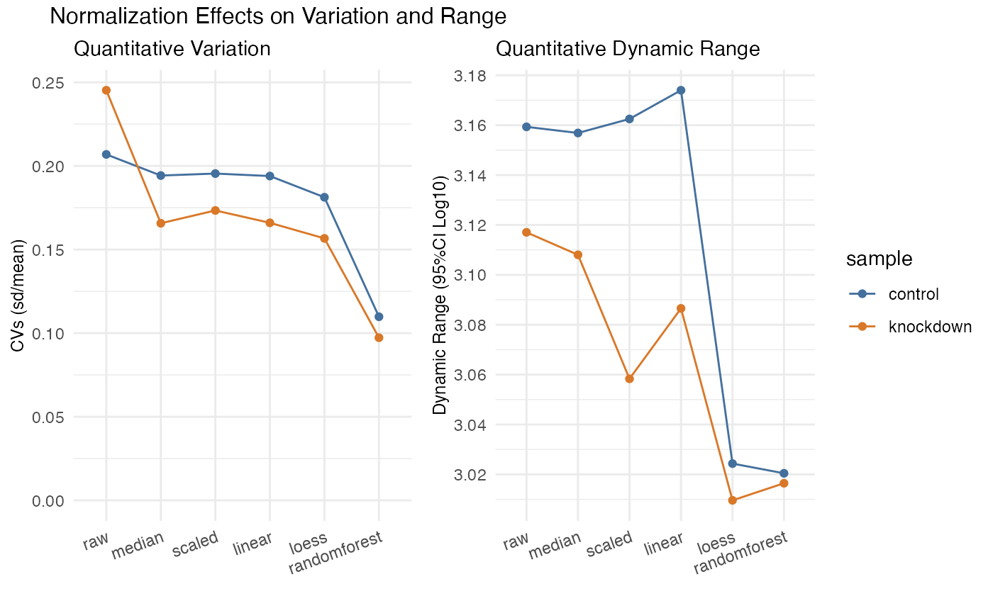

#> TableGrob (2 x 2) "arrange": 3 grobs
#>   z     cells    name               grob
#> 1 1 (2-2,1-1) arrange     gtable[layout]
#> 2 2 (2-2,2-2) arrange     gtable[layout]
#> 3 3 (1-1,1-2) arrange text[GRID.text.86]

PCA

rdata %>% plot_variation_pca()

Effect of Normalization on Dynamic Range

The effect randomforest has on the data is most noticable at the lower dynamic range, as seen in the plot below where the CVs for values under 10^6 in abundance have been dramatically reduced. If you are hunting for low abundant biomarkers, this method is highly recomended.

hela_proteins %>%
  normalize(.method = c('median', 'randomforest')) %>% 
  plot_dynamic_range()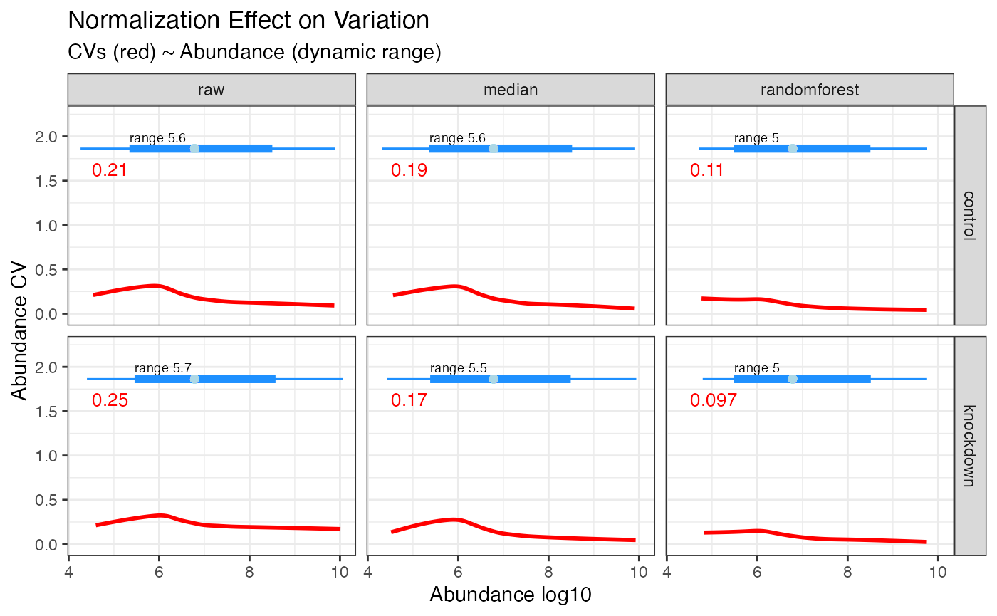
#> Warning in ggplot2::geom_point(ggplot2::aes(x = range_x, y = range_y), color = "lightblue"): All aesthetics have length 1, but the data has 30456 rows.
#> ℹ Did you mean to use `annotate()`?
#> Warning: Computation failed in `stat_binhex()`.
#> Computation failed in `stat_binhex()`.
#> Computation failed in `stat_binhex()`.
#> Computation failed in `stat_binhex()`.
#> Computation failed in `stat_binhex()`.
#> Computation failed in `stat_binhex()`.
#> Caused by error in `compute_group()`:
#> ! The package "hexbin" is required for `stat_bin_hex()`.

Normalization based on a subset

In addition to proteome wide normalization, a subset can be used as the basis for normalization, such as the case for spike-in quantitative analytes or the perhaps the bait protein in an immunoprecipitation experiment. This is accomplished with the same semantic syntax as with the subset() function and is reflected in the recorded operations. Be aware that using a regression from a smaller dynamic range than the full proteome may not predict well beyond the limts of the subset.

NOTE: while linear and svm can predict beyond the training set limits, loess can not.

NOTE: The randomforest normalization method, as implemented, requires the the prediction set size to match the training test size, and therefore is only applicable to normalization of the whole proteome. The limma normalization method also does not accept a subset for normalization. Both of these methods will be skipped if a subset is implemented.

rdata <- hela_proteins %>%
  normalize(description %like% 'ribosome',
            .method = c('median', 'linear', 'loess', 'svm')) 

rdata %>% plot_variation_cv()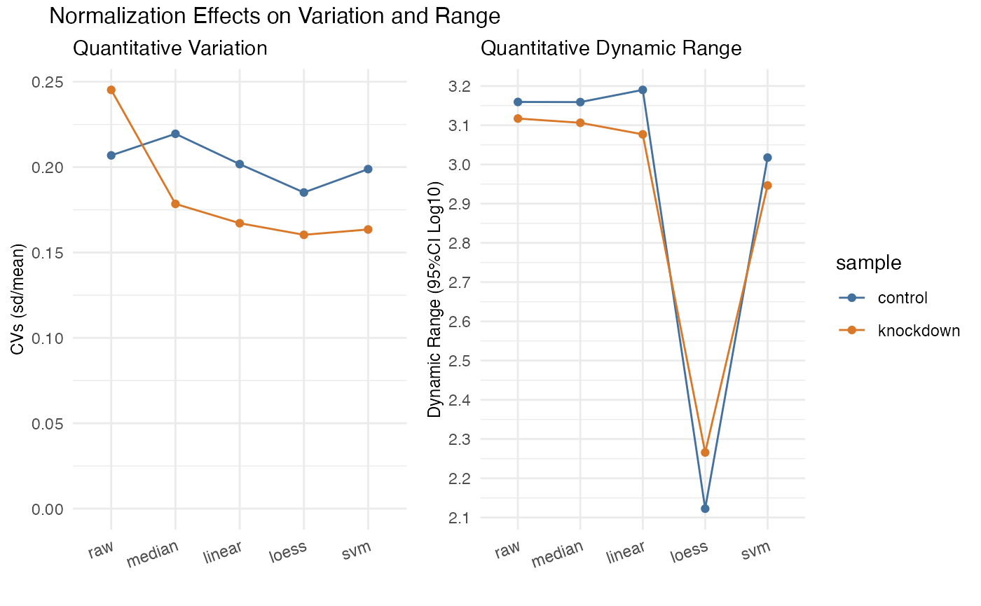

#> TableGrob (2 x 2) "arrange": 3 grobs
#>   z     cells    name                grob
#> 1 1 (2-2,1-1) arrange      gtable[layout]
#> 2 2 (2-2,2-2) arrange      gtable[layout]
#> 3 3 (1-1,1-2) arrange text[GRID.text.525]

rdata %>% plot_dynamic_range()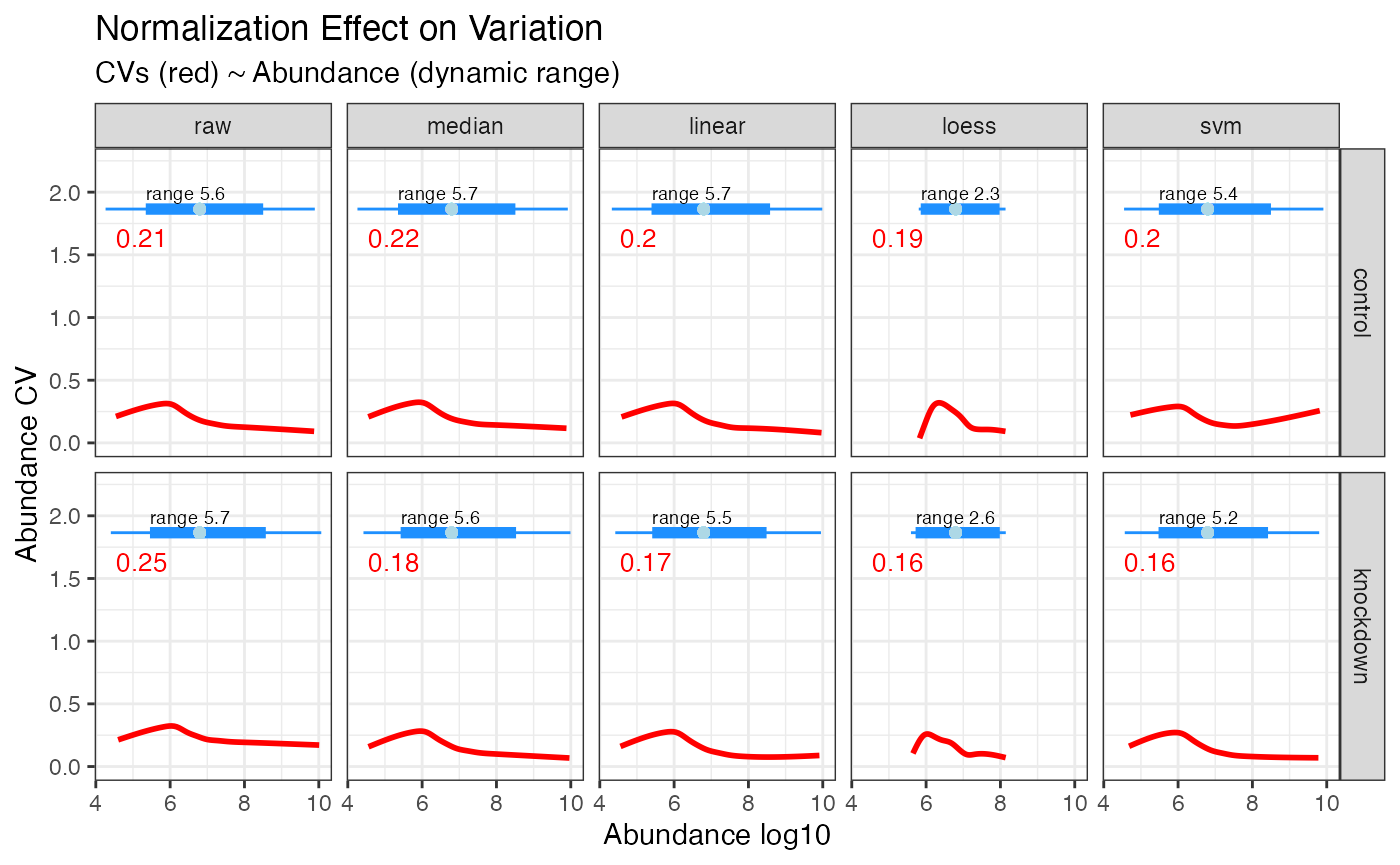
#> Warning in ggplot2::geom_point(ggplot2::aes(x = range_x, y = range_y), color = "lightblue"): All aesthetics have length 1, but the data has 49546 rows.
#> ℹ Did you mean to use `annotate()`?
#> Warning: Computation failed in `stat_binhex()`.
#> Computation failed in `stat_binhex()`.
#> Computation failed in `stat_binhex()`.
#> Computation failed in `stat_binhex()`.
#> Computation failed in `stat_binhex()`.
#> Computation failed in `stat_binhex()`.
#> Computation failed in `stat_binhex()`.
#> Computation failed in `stat_binhex()`.
#> Computation failed in `stat_binhex()`.
#> Computation failed in `stat_binhex()`.
#> Caused by error in `compute_group()`:
#> ! The package "hexbin" is required for `stat_bin_hex()`.

rdata %>% operations()
#> ℹ Data Transformations
#>   • Data files (p97KD_HCT116_proteins.xlsx) were imported as proteins from
#>   ProteomeDiscoverer
#> 
#>   • Data normalized via median, linear, loess, svm.
#> 
#>   • Data normalized using subset description %like% ribosome FALSE.
#> 
#>   • ... based on a subset of 17 out of 5346 identifiers
#> 
#>   • Normalization automatically selected as svm.

Developing Additional Methods

The normalization function can accommodate new methods fairly easily, but not without being tested and integrated with the package as a whole. This is due to the serial deployment of each normalization method and subsequent selection of the best method going forward. That could change in the future. For now lets walk through the process of adding a new method. And as always, reach out the the maintainers to have your method added to the package for others to use.

Where the normalization gets called

In the code base locate the file R > control_normalization.R, this is where the method gets applied. Note, near the bottom, the if() statements, specifically for median, this is where median normalization gets implemented.

## d:        the raw data for all samples
## dc_this:  the 'centered' data
## d_norm:   the output normalized data

if(m == 'median') {         d_norm <- d %>% normalize_median(dc_this)}

All normalization functions require two inputs, a table of all the raw values log2 transformed, and a table of grouped and ‘centered’ values to normalize against. This table can either be computed from the entire proteome or from a subset as demonstrated above.

## the log2 raw values

# A tibble: 30,157 × 4
   sample    replicate identifier abundance
   <chr>     <chr>     <chr>          <dbl>
 1 control   1         Q15149          29.9
 2 control   2         Q15149          30.0
 3 control   3         Q15149          29.9
 4 knockdown 1         Q15149          30.4
 5 knockdown 2         Q15149          30.0
 6 knockdown 3         Q15149          30.5
 ...

The normalization function

For the median normalization method, all samples will be adjusted such that their medians are aligned. Therefor, we need to take the median value of each sample, and the median of the medians, such that they all align.

normalize_median <- function(
    data = NULL,
    data_centered = NULL
){

  # visible bindings
  abundance <- NULL

  # compute the median shift
  data_centered <- data_centered %>%
    mutate(shift = median(abundance) - abundance)

  # apply the median shift and return the data
  data %>%
    left_join(data_centered,
              by = c('sample','replicate'),
              suffix = c("","_median")) %>%
    mutate(abundance_normalized = abundance + shift) %>%
    select(identifier, sample, replicate, abundance_normalized) %>%
    return()
}

Normalized data gets merged on return

The data, upon return to the controller function, has the abundance values converted back to non-log values, and merged into the main data object such that all abundance values are avaiable for future selection.

d_norm <- d_norm %>%
      dplyr::mutate(abundance_normalized = invlog2(abundance_normalized)) %>%
      dplyr::rename(abundance = abundance_normalized)

    data <- data %>% merge_quantitative(d_norm, m)
    
# A tibble: 42,330 × 6
   sample_id sample    replicate protein abundance_raw abundance_median
   <chr>     <chr>     <chr>     <chr>           <dbl>            <dbl>
 1 e9b20ea7  control   1         Q15149    1011259992.       999619474.
 2 ef79cc4c  control   2         Q15149    1093277593.      1106008756.
 3 eebba67b  control   3         Q15149     980809516.      1094113651.
 4 ebf4b0fe  knockdown 1         Q15149    1410445367.      1062933343.
 5 ea36dac9  knockdown 2         Q15149    1072305561.      1113989578.
 6 ecfd1822  knockdown 3         Q15149    1486561518.      1076375880.
 7 e9b20ea7  control   1         Q09666     659299359.       651710227.
 8 ef79cc4c  control   2         Q09666     717783135.       726141683.
 9 eebba67b  control   3         Q09666     612673576.       683450264.
10 ebf4b0fe  knockdown 1         Q09666    1000041657.       753646788.

hela_proteins %>% normalize(.method = 'median') %>% plot_normalization()
#> ℹ Normalizing quantitative data
#> ℹ ... using median shift
#> ✔ ... using median shift [150ms]
#> 
#> ℹ Selecting best normalization method
#> ✔ Selecting best normalization method ... done
#> 
#> ℹ  ... selected median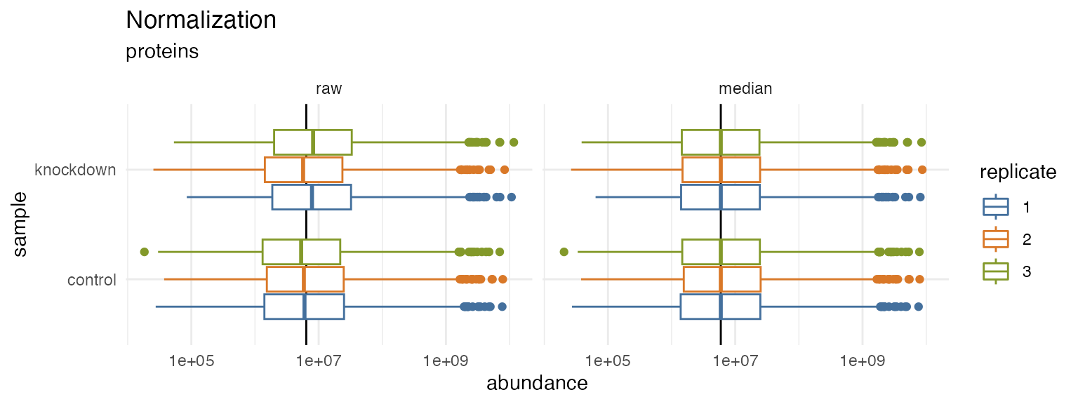

Check out some of the other normalization functions to see how they are implemented.