Protein Accounting
collapsing.RmdProtein accounting is an important aspect of quantiative proteomics. It consists of aggregating individual peptide measurements into a single reported protein. However, sequence homology make this a less than trivial process, as the LCMS process does not identify proteins specifically, rather their individual peptide segments. It is then up to the researcher to implement a method that infers the original protein content.
While the proteomics community at large has devised several schemes for protein accounting, not all methods are universally amenable. For example, when accounting for cellular differences between to cell states, it is often preferred to arrive at the minimal number of protein sequences that can explain the data. That means tossing aside identifiers to sequence variants - something researchers attempting to identify specific genes might like to retain. Furthermore, for researchers attempting to grasp if gene insertions are viable, gross summation of peptide abundances may miss nuances in sequence variations. These latter points are not well controlled for in platforms that cater for proteome wide discoveries. Therefor, we have attempted to provide several simple mechanisms that can apply to a variety of LCMS proteomics projects both larger proteome wide discoveries and smaller induced expression projects.
More sophisticated methods of protein accounting should utilize those current implementations, export the quantitative protein level data and then import into tidyproteomics.
NOTE: tidyproteomics allows you to group and summarize quantitative values for any annotation term, such as gene_name or even molecular_function giving you flexibility on how individual peptide values get summarized into larger observations. See Collapsing to Gene Name.
The inputs
assign_by
The collapse() function accommodates four methods for
accounting with the variable:
| Method | Description |
|---|---|
| all-possible | retain all protein assignments regardless of homology |
| non-homologous | retain all protein assignments, but only use quantitative values from peptides that identify a single unique protein. |
| razor-local | peptide will be assigned to the protein group with the largest number of total peptides identified within a sample group |
| razor-global | peptide will be assigned to the protein group with the largest number of total peptides identified globally |
top_n
this variable sets the number of peptide quantitative values to include in the final protein quantitative value.
split_abundance
a true/false variable, if true, will split abundances of razor-peptides by the proportional abundance between proteins. This method is experimental, has not been validated or peer-reviewed.
fasta_path can be provided to calculate iBAQ based values. However, currently this method only supports Tryptic based peptide accounting.
Examples
Here we import a data-object of ProteomeDiscoverer’s protein level accounting and investigate the difference between ProteomeDiscoverer’s protein accounting and that implemented by tidyproteomics.
# download the data
url_pro <- "https://data.caltech.edu/records/aevwq-2ps50/files/ProteomeDiscoverer_2.5_p97KD_HCT116_proteins.xlsx?download=1"
url_pep <- "https://data.caltech.edu/records/aevwq-2ps50/files/ProteomeDiscoverer_2.5_p97KD_HCT116_peptides.xlsx?download=1"

download.file(url_pro, destfile = "./data/pd_proteins.xlsx")
download.file(url_pep, destfile = "./data/pd_peptides.xlsx")

# import the data
pro_data <- "./data/pd_proteins.xlsx" %>% import('ProteomeDiscoverer', 'proteins')
pep_data <- "./data/pd_peptides.xlsx" %>% import('ProteomeDiscoverer', 'peptides')
Assign peptides by razor logic
pro_frompep_razor <- pep_data %>%
  collapse(assign_by = 'razor-global', top_n = Inf) %>%
  normalize(.method = c('median', 'linear', 'loess'))

pro_frompep_razor %>%
  summary("sample", destination = 'return') %>%
  select(c('sample', 'proteins', 'peptides', 'CVs')) %>%
  as.data.frame()
#>   sample proteins peptides  CVs
#> 1    ctl     7056    63622 0.14
#> 2 p97_kd     7056    63622 0.11
Check to see how the two results agree …
tbl_merged_razor <- pro_frompep_razor$quantitative %>%
  select('sample','replicate','protein', 'abundance_raw') %>%
  inner_join(pro_data$quantitative %>% select('sample','replicate','protein', 'abundance_raw'),
             by = c('sample','replicate','protein'),
             suffix = c("_tidyproteomics", "_proteomediscoverer"))

tbl_merged_razor %>%
  mutate(itentical_protein_abundances = abundance_raw_proteomediscoverer == abundance_raw_tidyproteomics) %>%
  filter(!is.na(itentical_protein_abundances)) %>%
  group_by(itentical_protein_abundances) %>%
  summarise(n = n(), .groups = 'drop') %>%
  mutate(r = paste(n / sum(n) * 100, "%")) %>%
  as.data.frame()
#>   itentical_protein_abundances     n                  r
#> 1                        FALSE 10187 34.2006311690056 %
#> 2                         TRUE 19599 65.7993688309944 %
A quick plot for visualizing the
tbl_merged_razor %>%
  mutate(sample_rep = paste(sample, replicate)) %>%
  ggplot(aes(abundance_raw_proteomediscoverer, abundance_raw_tidyproteomics)) +
  geom_abline(color='red') +
  geom_point(alpha = .67) +
  scale_x_log10() +
  scale_y_log10() +
  facet_wrap(~sample_rep)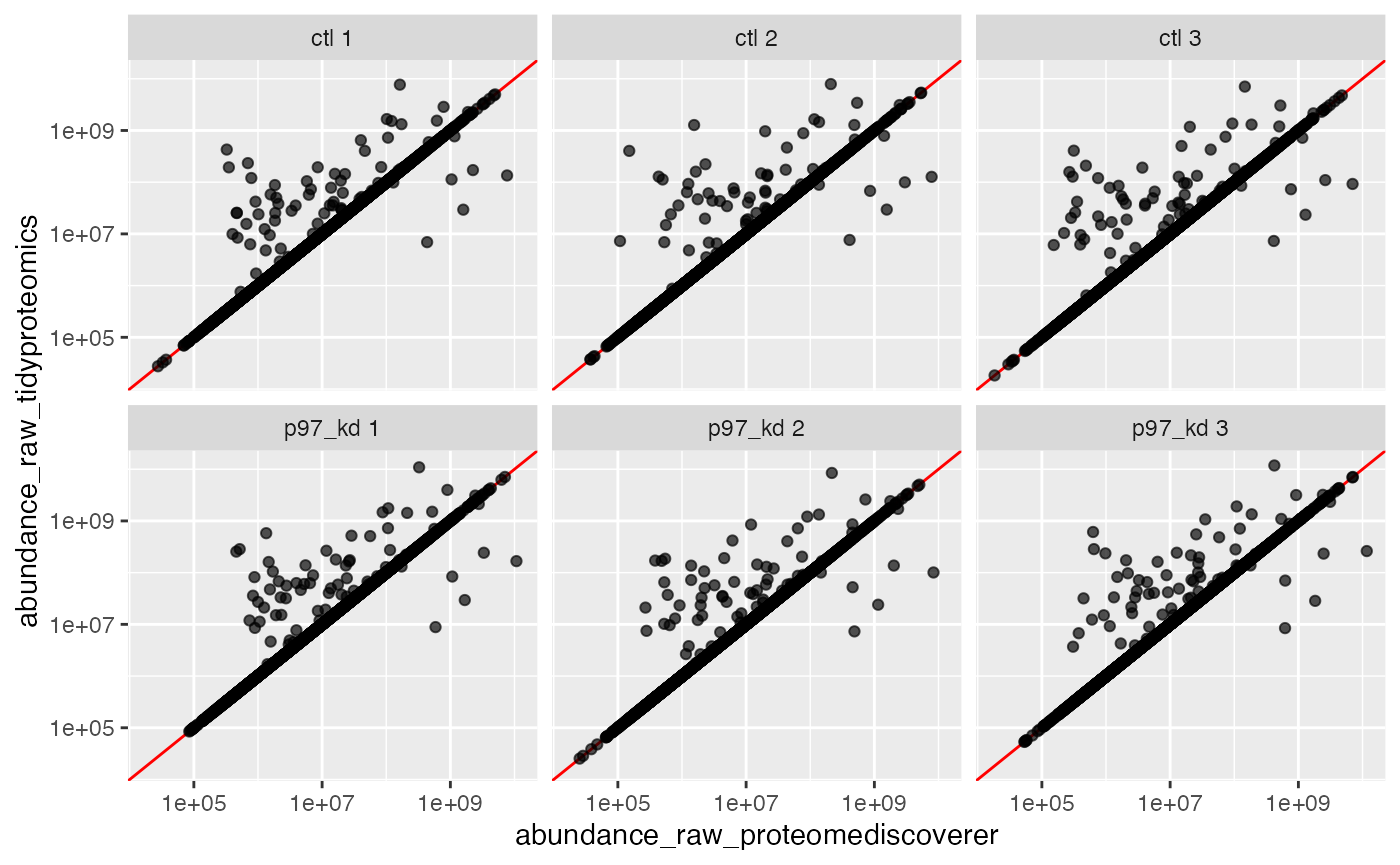
Lets look at a few examples of outliers …
tbl_merged_razor %>%
  filter(abundance_raw_proteomediscoverer != abundance_raw_tidyproteomics) %>% as.data.frame() %>% head()
#>   sample replicate protein abundance_raw_tidyproteomics
#> 1    ctl         1  F6RH32                     37467.02
#> 2    ctl         1  A7E2V4                     41468.92
#> 3    ctl         1  P78560                     66449.06
#> 4    ctl         1  Q7Z7G8                     68671.84
#> 5    ctl         1  Q6JQN1                     76441.32
#> 6    ctl         1  Q86W10                     88252.36
#>   abundance_raw_proteomediscoverer
#> 1                         56190.43
#> 2                         35352.48
#> 3                        140849.52
#> 4                        124222.47
#> 5                         89400.16
#> 6                         73711.15
We will take the protein P45983 to examine …
pep_P45983 <- pep_data$quantitative %>%
  filter(!is.na(abundance_raw)) %>%
  filter(sample == 'p97_kd', replicate == 1) %>%
  filter(protein == 'P45983')

pep_data$quantitative %>%
  filter(!is.na(abundance_raw)) %>%
  filter(sample == 'p97_kd', replicate == 1) %>%
  filter(peptide %in% pep_P45983$peptide) %>%
  group_by(peptide, modifications) %>%
  summarise(
    proteins = paste(protein, collapse = "; "),
    abundance_raw = unique(abundance_raw)
  ) %>%
  as.data.frame()
#>                       peptide           modifications
#> 1                    EHTIEEWK                    <NA>
#> 2                    IIDFGLAR                    <NA>
#> 3 ISVDEALQHPYINVWYDPSEAEAPPPK                    <NA>
#> 4               MSYLLYQMLCGIK 1xCarbamidomethyl [C10]
#> 5              VIEQLGTPCPEFMK  1xCarbamidomethyl [C9]
#> 6                    YAGYSFEK                    <NA>
#>                                         proteins abundance_raw
#> 1                                         P45983      278901.6
#> 2 O15264; Q86YV6; P45984; P53778; Q16539; P45983     2796395.2
#> 3                                         P45983      355809.2
#> 4                                 P45984; P45983      137644.7
#> 5                                         P45983      601605.8
#> 6                                         P45983      399617.4
Here we see that P45983 yielded 5 peptides, 2 of which are shared. In the outlier table we see that ProteomeDiscoverer excluded all razor peptides from the protein quantitation. And if we dig further, we find that the peptide IIDFGLAR by razor definition belongs to the protein Q16539, while the peptide MSYLLYQMLCGIK can be assigned to P45983, thus giving us the larger value shown in the outlier table.
pep_data$quantitative %>%
  filter(!is.na(abundance_raw)) %>%
  filter(sample == 'p97_kd', replicate == 1) %>%
  filter(protein %in% c('O15264','Q86YV6','P45984','P53778','Q16539','P45983')) %>%
  group_by(protein) %>%
  summarise(
    n_peptides = length(unique(peptide))
  ) %>%
  arrange(desc(n_peptides)) %>%
  as.data.frame()
#>   protein n_peptides
#> 1  Q16539          7
#> 2  P45983          6
#> 3  P45984          3
#> 4  O15264          2
#> 5  Q86YV6          2
#> 6  P53778          1
Assign by excluding homologous peptides
That means the ProteomeDiscoverer method for protein accounting excluded the abundance measurement from all razor peptides. Lets try to replicate that as well.
pro_frompep_nonhom <- pep_data %>%
  collapse(assign_by = 'non-homologous', top_n = Inf) %>%
  normalize(.method = c('median', 'linear', 'loess'))

pro_frompep_nonhom %>%
  summary("sample", destination = 'return') %>%
  select(c('sample', 'proteins', 'peptides', 'CVs')) %>%
  as.data.frame()
#>   sample proteins peptides  CVs
#> 1    ctl     7056    63622 0.14
#> 2 p97_kd     7056    63622 0.12
Check to see how the two results agree …
tbl_merged_nonhom <- pro_frompep_nonhom$quantitative %>% select('sample','replicate','protein', 'abundance_raw') %>%
  inner_join(pro_data$quantitative %>% select('sample','replicate','protein', 'abundance_raw'),
             by = c('sample','replicate','protein'),
             suffix = c("_tidyproteomics", "_proteomediscoverer"))

tbl_merged_nonhom %>%
  mutate(itentical_protein_abundances = abundance_raw_proteomediscoverer == abundance_raw_tidyproteomics) %>%
  filter(!is.na(itentical_protein_abundances)) %>%
  group_by(itentical_protein_abundances) %>%
  summarise(n = n(), .groups = 'drop') %>%
  mutate(r = paste(n / sum(n) * 100, "%")) %>%
  as.data.frame()
#>   itentical_protein_abundances     n                  r
#> 1                        FALSE 11882 40.2043716586587 %
#> 2                         TRUE 17672 59.7956283413413 %
A quick plot for visualizing the
tbl_merged_nonhom %>%
  mutate(sample_rep = paste(sample, replicate)) %>%
  ggplot(aes(abundance_raw_proteomediscoverer, abundance_raw_tidyproteomics)) +
  geom_abline(color='red') +
  geom_point(alpha = .67) +
  scale_x_log10() +
  scale_y_log10() +
  facet_wrap(~sample_rep)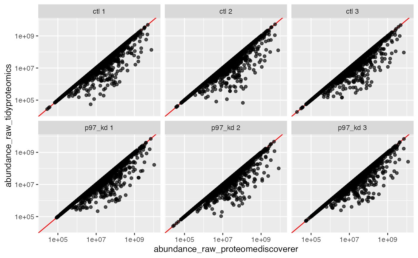
Interesting, we now show that P45983 agrees with ProteomeDiscoverer, yet obviously several others do not
tbl_merged_nonhom %>% filter(protein == 'P45983') %>%
  as.data.frame()
#>   sample replicate protein abundance_raw_tidyproteomics
#> 1    ctl         1  P45983                     703721.1
#> 2 p97_kd         1  P45983                    1635934.1
#> 3    ctl         2  P45983                     535040.5
#> 4    ctl         3  P45983                     494210.7
#> 5 p97_kd         2  P45983                    1409719.2
#> 6 p97_kd         3  P45983                    2219424.9
#>   abundance_raw_proteomediscoverer
#> 1                         494210.7
#> 2                        1635934.1
#> 3                         535040.5
#> 4                         703721.1
#> 5                        1409719.2
#> 6                        2219424.9
Lets look at a few examples of outliers …
tbl_merged_nonhom %>%
  filter(abundance_raw_proteomediscoverer != abundance_raw_tidyproteomics) %>%
  head(3) %>%
  as.data.frame()
#>   sample replicate protein abundance_raw_tidyproteomics
#> 1    ctl         1  F6RH32                     37467.02
#> 2    ctl         1  A7E2V4                     41468.92
#> 3    ctl         1  P78560                     66449.06
#>   abundance_raw_proteomediscoverer
#> 1                         56190.43
#> 2                         35352.48
#> 3                        140849.52
We will take the protein Q96LR5 to examine …
pep_Q96LR5 <- pep_data$quantitative %>%
  filter(!is.na(abundance_raw)) %>%
  filter(sample == 'p97_kd', replicate == 1) %>%
  filter(protein == 'Q96LR5')

pep_data$quantitative %>%
  filter(!is.na(abundance_raw)) %>%
  filter(sample == 'p97_kd', replicate == 1) %>%
  filter(peptide %in% pep_Q96LR5$peptide) %>%
  group_by(peptide, modifications) %>%
  summarise(
    proteins = paste(protein, collapse = "; "),
    abundance_raw = unique(abundance_raw)
  ) %>%
  as.data.frame()
#> `summarise()` has grouped output by 'peptide'. You can override using the
#> `.groups` argument.
#>              peptide               modifications               proteins
#> 1        DNWSPALTISK                        <NA> Q96LR5; P51965; Q969T4
#> 2 ELAEITLDPPPNCSAGPK     1xCarbamidomethyl [C13]         Q96LR5; Q969T4
#> 3 IYHCNINSQGVICLDILK 2xCarbamidomethyl [C4; C13] Q96LR5; P51965; Q969T4
#> 4  VDDSPSTSGGSSDGDQR                        <NA>                 Q96LR5
#>   abundance_raw
#> 1     6026133.5
#> 2     1561461.0
#> 3     1263053.9
#> 4      195230.2
A quick check on the peptide sum and it appears that ProteomeDiscoverer ignored razor-peptides all together for this protein
pep_data$quantitative %>%
  filter(!is.na(abundance_raw)) %>%
  filter(sample == 'p97_kd', replicate == 1) %>%
  filter(peptide %in% pep_Q96LR5$peptide) %>%
  group_by(peptide, modifications) %>%
  summarise(
    proteins = paste(protein, collapse = "; "),
    abundance_raw = unique(abundance_raw),
    .groups = 'drop'
  ) %>%
  summarise(abundance_sum = sum(abundance_raw)) %>%
  as.data.frame()
#>   abundance_sum
#> 1       9045879
If we examine the other proteins in that group for all the peptides that may be shared …
get_peptides <- pep_data$quantitative %>%
  filter(!is.na(abundance_raw)) %>%
  filter(sample == 'p97_kd', replicate == 1) %>%
  filter(protein %in% c('Q96LR5','P51965','Q969T4'))

pep_data$quantitative %>%
  filter(!is.na(abundance_raw)) %>%
  filter(sample == 'p97_kd', replicate == 1) %>%
  filter(peptide %in% get_peptides$peptide) %>%
  group_by(peptide, modifications) %>%
  summarise(
    proteins = paste(protein, collapse = "; "),
    abundance_raw = unique(abundance_raw)
  ) %>%
  as.data.frame()
#> `summarise()` has grouped output by 'peptide'. You can override using the
#> `.groups` argument.
#>              peptide               modifications               proteins
#> 1        DNWSPALTISK                        <NA> Q96LR5; P51965; Q969T4
#> 2      DPAAPEPEEQEER                        <NA>                 Q969T4
#> 3 ELADITLDPPPNCSAGPK     1xCarbamidomethyl [C13]                 P51965
#> 4 ELAEITLDPPPNCSAGPK     1xCarbamidomethyl [C13]         Q96LR5; Q969T4
#> 5 IYHCNINSQGVICLDILK 2xCarbamidomethyl [C4; C13] Q96LR5; P51965; Q969T4
#> 6  VDDSPSTSGGSSDGDQR                        <NA>                 Q96LR5
#>   abundance_raw
#> 1     6026133.5
#> 2      185996.9
#> 3     1543880.8
#> 4     1561461.0
#> 5     1263053.9
#> 6      195230.2
… we see that ProteomeDiscoverer actually assigned the abundances of razor-peptides. And if we check our results from the merged razor data we find that to be correct.
tbl_merged_razor %>%
  filter(sample == 'p97_kd', replicate == 1) %>%
  filter(protein %in% c('Q96LR5','P51965','Q969T4')) %>%
  as.data.frame()
#>   sample replicate protein abundance_raw_tidyproteomics
#> 1 p97_kd         1  Q969T4                     185996.9
#> 2 p97_kd         1  P51965                    1543880.8
#> 3 p97_kd         1  Q96LR5                    9045878.5
#>   abundance_raw_proteomediscoverer
#> 1                         185996.9
#> 2                        1543880.8
#> 3                        9045878.5
Collapsing to Gene Name
Alternatively, peptide level data can be collapsed to any Annotation
term, in this case we will collapse to gene_name after adding the
annotations to the peptide data object. See
vignette("annotating").
library(tidyr)

gene_data <- pep_data %>%
  collapse(collapse_to = 'gene_name', fasta_path = "uniprot_human-20398_20220920.fasta")
gene_data %>% plot_counts()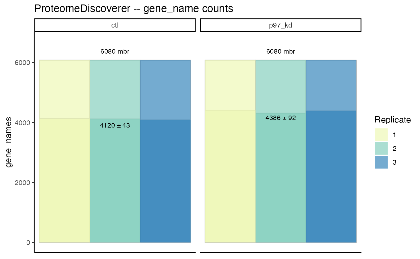
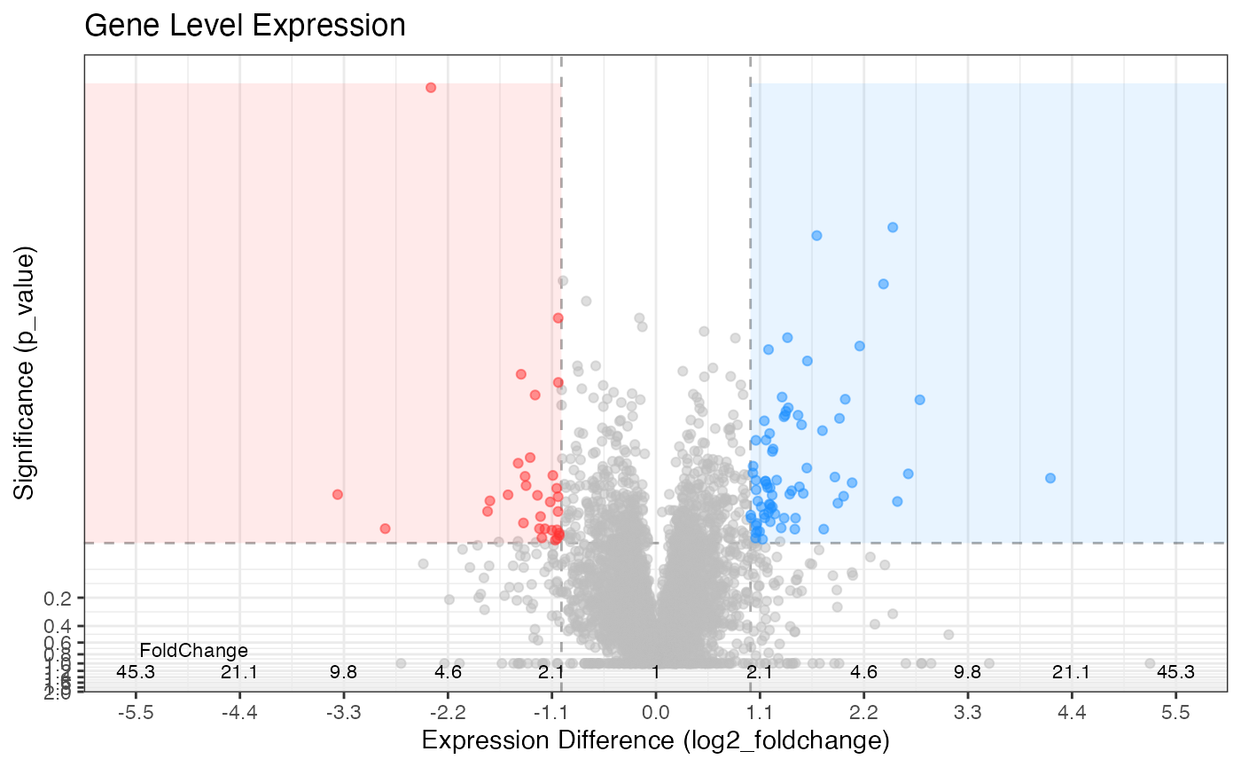
gene_data %>%
  normalize(.method = 'linear') %>%
  expression(p97_kd/ctl) %>%
  plot_volcano(p97_kd/ctl, significance_column = 'p_value') +
  labs(title = "Gene Level Expression")
#> ℹ Normalizing quantitative data
#> ℹ ... using linear regression
#> ✔ ... using linear regression [214ms]
#>
#> ℹ Selecting best normalization method
#> ✔ Selecting best normalization method ... done
#>
#> ℹ  ... selected linear
#> ℹ .. expression::t_test testing p97_kd / ctl
#> ✔ .. expression::t_test testing p97_kd / ctl [3.2s]
#>
#> [1] 7.971310e-07 4.888556e-02
#> Warning: ggrepel: 84 unlabeled data points (too many overlaps). Consider
#> increasing max.overlaps