Annotating
annotating.RmdAnnotating data
As a part of the Tidyproteomics workflow, we need to update the
gene_name and description annotated terms in
the data imported from FragPipe. To accomplish this, we will use
information from a parsed FASTA file. The parsed FASTA file should
contain three columns: protein identifier,
term, and annotation.
Updating the gene_name and description
annotated terms will allow for easier interpretation and analysis of the
data. The gene_name and description attributes
provide crucial information about the protein, such as its function and
biological role. By updating these attributes with information from the
FASTA file, we can ensure that our data is accurate and informative.
The process of updating the gene_name and
description annotated terms is simple. First, we will parse
the FASTA file to extract the necessary information. Then, we will use
this information to update the corresponding attributes in the imported
data from FragPipe.
It is important to note that the parsed FASTA file must contain
accurate and up-to-date information. If the information in the FASTA
file is outdated or incorrect, the updated gene_name and
description attributes will also be incorrect. Therefore,
it is essential to verify the accuracy of the FASTA file before using it
to update the imported data from FragPipe.
library(tidyverse)
library(tidyproteomics)

# download the data
url <- "https://ftp.ebi.ac.uk/pride-archive/2016/06/PXD004163/Yan_miR_Protein_table.flatprottable.txt"
download.file(url, destfile = "./data/combined_protein.tsv", method = "auto")

# import the data
data_prot <- "./data/combined_protein.tsv" %>% import('FragPipe', 'proteins')
From a FASTA File
Read in a FASTA file using some “un-exposed” methods in the
tidyproteomics package.
data_fasta <- "~/Local/data/fasta/uniprot_human-20398_20220920.fasta" %>%
  tidyproteomics:::fasta_parse(as = "data.frame") %>%
  select(protein = accession, gene_name, description) %>%
  pivot_longer(
    cols = c('gene_name', 'description'),
    names_to = 'term',
    values_to = 'annotation'
  )

data_fasta %>% filter(protein %in% c('P68431', 'P62805'))
#> # A tibble: 4 × 3
#>   protein term        annotation
#>   <chr>   <chr>       <chr>
#> 1 P62805  gene_name   H4-16
#> 2 P62805  description Histone H4
#> 3 P68431  gene_name   H3C12
#> 4 P68431  description Histone H3.1
Notice the gene_name annotations are different from the
FASTA than from the FragPipe outoput.
data_prot$annotations %>% filter(protein %in% c('P68431', 'P62805'))
#> # A tibble: 4 × 3
#>   protein term        annotation
#>   <chr>   <chr>       <chr>
#> 1 P62805  gene_name   H4C1
#> 2 P62805  description Histone H4
#> 3 P68431  gene_name   H3C1
#> 4 P68431  description Histone H3.1
We can merge the annotations,
data_new_merged <- data_prot %>% annotate(data_fasta, duplicates = 'merge')

data_new_merged$annotations %>% filter(protein %in% c('P68431', 'P62805'))
#> # A tibble: 4 × 3
#>   protein term        annotation
#>   <chr>   <chr>       <chr>
#> 1 P62805  description Histone H4
#> 2 P62805  gene_name   H4C1; H4-16
#> 3 P68431  description Histone H3.1
#> 4 P68431  gene_name   H3C1; H3C12
Or we can replace the annotations,
data_new_replaced <- data_prot %>% annotate(data_fasta, duplicates = 'replace')

data_new_replaced$annotations %>% filter(protein %in% c('P68431', 'P62805'))
#> # A tibble: 4 × 3
#>   protein term        annotation
#>   <chr>   <chr>       <chr>
#> 1 P62805  description Histone H4
#> 2 P62805  gene_name   H4-16
#> 3 P68431  description Histone H3.1
#> 4 P68431  gene_name   H3C12
GO Annotations
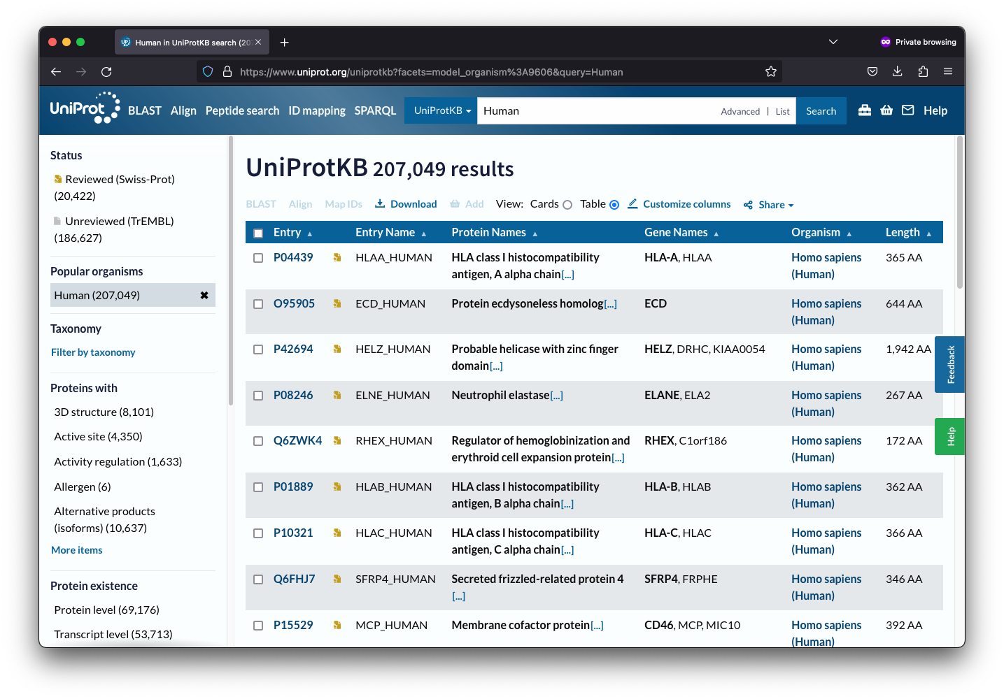
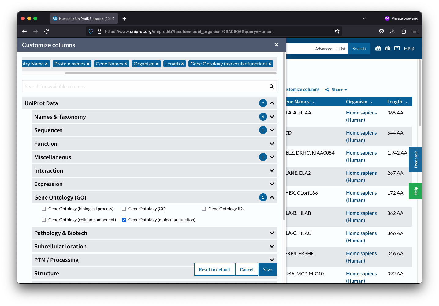
To obtain GO annotations, you can visit UniProt’s website and search for the proteins of interest, such as human proteins. Once you have found the proteins, you will need to select the “Customize columns” option to access several options, including Gene Ontology.
After selecting Gene Ontology, you will need to choose the desired values, such as molecular function, by clicking on them. Once you have selected your desired values, click on the “Save” button to save your changes.
Finally, you can download the table as a TSV file by clicking on the “Download” button. This file will contain all the information you need about your selected proteins, making it easier to analyze and interpret the data.
Now that you know how to obtain GO annotations, you can use this information to enhance your research and analysis. UniProt’s website is a valuable resource for obtaining information about proteins, and the ability to customize columns and select desired values makes it even more useful for researchers and scientists.
Read in the TSV file from the downloaded UniProt table.
data_go <- "~/Local/data/uniprotkb/uniprotkb_human_AND_reviewed_true_AND_m_2023_10_10.tsv" %>% read_tsv()

data_go
#> # A tibble: 20,426 × 8
#>    Entry      Reviewed `Entry Name` `Protein names` `Gene Names` Organism Length
#>    <chr>      <chr>    <chr>        <chr>           <chr>        <chr>     <dbl>
#>  1 A0A087X1C5 reviewed CP2D7_HUMAN  Putative cytoc… CYP2D7       Homo sa…    515
#>  2 A0A0B4J2F0 reviewed PIOS1_HUMAN  Protein PIGBOS… PIGBOS1      Homo sa…     54
#>  3 A0A0B4J2F2 reviewed SIK1B_HUMAN  Putative serin… SIK1B        Homo sa…    783
#>  4 A0A0C5B5G6 reviewed MOTSC_HUMAN  Mitochondrial-… MT-RNR1      Homo sa…     16
#>  5 A0A0K2S4Q6 reviewed CD3CH_HUMAN  Protein CD300H… CD300H       Homo sa…    201
#>  6 A0A0U1RRE5 reviewed NBDY_HUMAN   Negative regul… NBDY LINC01… Homo sa…     68
#>  7 A0A1B0GTW7 reviewed CIROP_HUMAN  Ciliated left-… CIROP LMLN2  Homo sa…    788
#>  8 A0AV02     reviewed S12A8_HUMAN  Solute carrier… SLC12A8 CCC9 Homo sa…    714
#>  9 A0AV96     reviewed RBM47_HUMAN  RNA-binding pr… RBM47        Homo sa…    593
#> 10 A0AVF1     reviewed IFT56_HUMAN  Intraflagellar… IFT56 TTC26  Homo sa…    554
#> # ℹ 20,416 more rows
#> # ℹ 1 more variable: `Gene Ontology (molecular function)` <chr>
We just need to tidy up that data a bit and get it into the format needed for attaching the annotations.
data_go <- data_go %>%
  select(protein = Entry,
         molecular_function = `Gene Ontology (molecular function)`) %>%
  # separate the GO terms so we get 1/row
  separate_rows(molecular_function, sep="\\;\\s") %>%
  # remove the [GO:accession]
  mutate(molecular_function = sub("\\s\\[.+", "", molecular_function)) %>%
  # pivot to the needed format
  pivot_longer(molecular_function,
               names_to = 'term',
               values_to = 'annotation')

data_go
#> # A tibble: 61,535 × 3
#>    protein    term               annotation
#>    <chr>      <chr>              <chr>
#>  1 A0A087X1C5 molecular_function aromatase activity
#>  2 A0A087X1C5 molecular_function heme binding
#>  3 A0A087X1C5 molecular_function iron ion binding
#>  4 A0A087X1C5 molecular_function oxidoreductase activity, acting on paired dono…
#>  5 A0A0B4J2F0 molecular_function NA
#>  6 A0A0B4J2F2 molecular_function ATP binding
#>  7 A0A0B4J2F2 molecular_function magnesium ion binding
#>  8 A0A0B4J2F2 molecular_function protein serine kinase activity
#>  9 A0A0B4J2F2 molecular_function protein serine/threonine kinase activity
#> 10 A0A0C5B5G6 molecular_function DNA binding
#> # ℹ 61,525 more rows
Looks great!
data_new_go <- data_prot %>% annotate(data_go)

data_new_go$annotations %>% filter(protein %in% c('P68431', 'P62805'))
#> # A tibble: 6 × 3
#>   protein term               annotation
#>   <chr>   <chr>              <chr>
#> 1 P62805  description        Histone H4
#> 2 P62805  gene_name          H4C1
#> 3 P62805  molecular_function structural constituent of chromatin
#> 4 P68431  description        Histone H3.1
#> 5 P68431  gene_name          H3C1
#> 6 P68431  molecular_function structural constituent of chromatin
Take it for a test drive by subsetting the data based on a specific annotation term.
data_new_go %>%
subset(molecular_function == 'structural constituent of chromatin')
#> Origin FragPipe
#> proteins (23.96 kB)
#> Composition 6 files
#> 2 samples (control, knockdown)
#> Quantitation 14 proteins
#> 2.7 log10 dynamic range
#> 16.7% missing values
#> *imputed
#> Accounting (3) num_psms num_psms_unique imputed
#> Annotations (3) molecular_function description gene_name
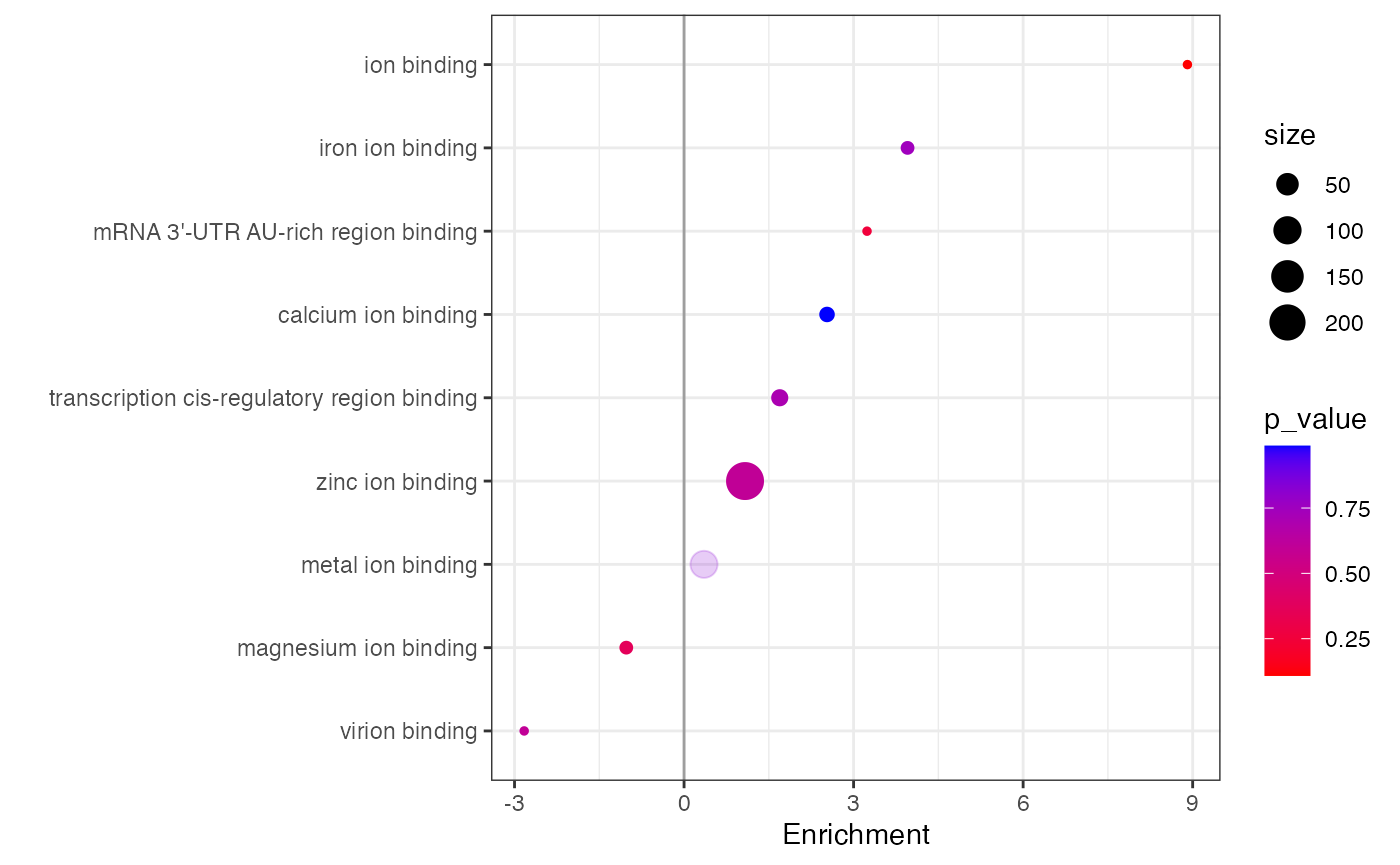
#> An enrichment plot for “ion binding” for the annotation
molecular_function.
data_new_go %>%
  subset(molecular_function %like% 'ion binding') %>%
  expression(knockdown/control) %>%
  enrichment(knockdown/control,
             .terms = 'molecular_function',
             .method = 'wilcoxon') %>%
  plot_enrichment(
    knockdown/control,
    .term = 'molecular_function',
    significance_max = 1
  )